This article reviews TAR 1.0, 2.0, and the new TAR 3.0 workflow.  It then compares performance on seven categorization tasks of varying prevalence and difficulty.  You may find it useful to read my article on gain curves before reading this one.

In some circumstances it may be acceptable to produce documents without reviewing all of them.  Perhaps it is expected that there are no privileged documents among the custodians involved, or maybe it is believed that potentially privileged documents will be easy to find via some mechanism like analyzing email senders and recipients.  Maybe there is little concern that trade secrets or evidence of bad acts unrelated to the litigation will be revealed if some non-relevant documents are produced.  In such situations you are faced with a dilemma when choosing a predictive coding workflow.  The TAR 1.0 workflow allows documents to be produced without review, so there is potential for substantial savings if TAR 1.0 works well for the case in question, but TAR 1.0 sometimes doesn’t work well, especially when prevalence is low.  TAR 2.0 doesn’t really support producing documents without reviewing them, but it is usually much more efficient than TAR 1.0 if all documents that are predicted to be relevant will be reviewed, especially if the task is difficult or prevalence is low.

TAR 1.0 involves a fair amount of up-front investment in reviewing control set documents and training documents before you can tell whether it is going to work well enough to produce a substantial number of documents without reviewing them.  If you find that TAR 1.0 isn’t working well enough to avoid reviewing documents that will be produced (too many non-relevant documents would slip into the production) and you resign yourself to reviewing everything that is predicted to be relevant, you’ll end up reviewing more documents with TAR 1.0 than you would have with TAR 2.0.  Switching from TAR 1.0 to TAR 2.0 midstream is less efficient than starting with TAR 2.0. Whether you choose TAR 1.0 or TAR 2.0, it is possible that you could have done less document review if you had made the opposite choice (if you know up front that you will have to review all documents that will be produced due to the circumstances of the case, TAR 2.0 is almost certainly the better choice as far as efficiency is concerned).

TAR 3.0 solves the dilemma by providing high efficiency regardless of whether or not you end up reviewing all of the documents that will be produced.  You don’t have to guess which workflow to use and suffer poor efficiency if you are wrong about whether or not producing documents without reviewing them will be feasible.  Before jumping into the performance numbers, here is a summary of the workflows (you can find some related animations and discussion in the recording of my recent webinar):

TAR 1.0 involves a training phase followed by a review phase with a control set being used to determine the optimal point when you should switch from training to review.  The system no longer learns once the training phase is completed.  The control set is a random set of documents that have been reviewed and marked as relevant or non-relevant.  The control set documents are not used to train the system.  They are used to assess the system’s predictions so training can be terminated when the benefits of additional training no longer outweigh the cost of additional training.  Training can be with randomly selected documents, known as Simple Passive Learning (SPL), or it can involve documents chosen by the system to optimize learning efficiency, known as Simple Active Learning (SAL).

TAR 2.0 uses an approach called Continuous Active Learning (CAL), meaning that there is no separation between training and review–the system continues to learn throughout.  While many approaches may be used to select documents for review, a significant component of CAL is many iterations of predicting which documents are most likely to be relevant, reviewing them, and updating the predictions.  Unlike TAR 1.0, TAR 2.0 tends to be very efficient even when prevalence is low.  Since there is no separation between training and review, TAR 2.0 does not require a control set.  Generating a control set can involve reviewing a large (especially when prevalence is low) number of non-relevant documents, so avoiding control sets is desirable.

TAR 3.0 requires a high-quality conceptual clustering algorithm that forms narrowly focused clusters of fixed size in concept space.  It applies the TAR 2.0 methodology to just the cluster centers, which ensures that a diverse set of potentially relevant documents are reviewed.  Once no more relevant cluster centers can be found, the reviewed cluster centers are used as training documents to make predictions for the full document population.  There is no need for a control set–the system is well-trained when no additional relevant cluster centers can be found. Analysis of the cluster centers that were reviewed provides an estimate of the prevalence and the number of non-relevant documents that would be produced if documents were produced based purely on the predictions without human review.  The user can decide to produce documents (not identified as potentially privileged) without review, similar to SAL from TAR 1.0 (but without a control set), or he/she can decide to review documents that have too much risk of being non-relevant (which can be used as additional training for the system, i.e., CAL).  The key point is that the user has the info he/she needs to make a decision about how to proceed after completing review of the cluster centers that are likely to be relevant, and nothing done before that point becomes invalidated by the decision (compare to starting with TAR 1.0, reviewing a control set, finding that the predictions aren’t good enough to produce documents without review, and then switching to TAR 2.0, which renders the control set virtually useless).

The table below shows the amount of document review required to reach 75% recall for seven categorization tasks with widely varying prevalence and difficulty.  Performance differences between CAL and non-CAL approaches tend to be larger if a higher recall target is chosen.  The document population is 100,000 news articles without dupes or near-dupes.  “Min Total Review” is the number of documents requiring review (training documents and control set if applicable) if all documents predicted to be relevant will be produced without review.  “Max Total Review” is the number of documents requiring review if all documents predicted to be relevant will be reviewed before production.  None of the results include review of statistical samples used to measure recall, which would be the same for all workflows.

	Task	1	2	3	4	5	6	7
	Prevalence	6.9%	4.1%	2.9%	1.1%	0.68%	0.52%	0.32%
TAR 1.0 SPL	Control Set	300	500	700	1,800	3,000	3,900	6,200
	Training (Random)	1,000	300	6,000	3,000	1,000	4,000	12,000
	Review Phase	9,500	4,400	9,100	4,400	900	9,800	2,900
	Min Total Review	1,300	800	6,700	4,800	4,000	7,900	18,200
	Max Total Review	10,800	5,200	15,800	9,200	4,900	17,700	21,100
TAR 3.0 SAL	Training (Cluster Centers)	400	500	600	300	200	500	300
	Review Phase	8,000	3,000	12,000	4,200	900	8,000	7,300
	Min Total Review	400	500	600	300	200	500	300
	Max Total Review	8,400	3,500	12,600	4,500	1,100	8,500	7,600
TAR 3.0 CAL	Training (Cluster Centers)	400	500	600	300	200	500	300
	Training + Review	7,000	3,000	6,700	2,400	900	3,300	1,400
	Total Review	7,400	3,500	7,300	2,700	1,100	3,800	1,700

The size of the control set for TAR 1.0 was chosen so that it would contain approximately 20 relevant documents, so low prevalence requires a large control set.  Note that the control set size was chosen based on the assumption that it would be used only to measure changes in prediction quality.  If the control set will be used for other things, such as recall estimation, it needs to be larger.

The number of random training documents used in TAR 1.0 was chosen to minimize the Max Total Review result (see my article on gain curves for related discussion).  This minimizes total review cost if all documents predicted to be relevant will be reviewed and if the cost of reviewing documents in the training phase and review phase are the same.  If training documents will be reviewed by an expensive subject matter expert and the review phase will be performed by less expensive reviewers, the optimal amount of training will be different.  If documents predicted to be relevant won’t be reviewed before production, the optimal amount of training will also be different (and more subjective), but I kept the training the same when computing Min Total Review values.

The optimal number of training documents for TAR 1.0 varied greatly for different tasks, ranging from 300 to 12,000.  This should make it clear that there is no magic number of training documents that is appropriate for all projects.  This is also why TAR 1.0 requires a control set–the optimal amount of training must be measured.

The results labeled TAR 3.0 SAL come from terminating learning once the review of cluster centers is complete, which is appropriate if documents will be produced without review (Min Total Review).  The Max Total Review value for TAR 3.0 SAL tells you how much review would be required if you reviewed all documents predicted to be relevant but did not allow the system to learn from that review, which is useful to compare to the TAR 3.0 CAL result where learning is allowed to continue throughout.  In some cases where the categorization task is relatively easy (tasks 2 and 5) the extra learning from CAL has no benefit unless the target recall is very high.  In other cases CAL reduces review significantly.

I have not included TAR 2.0 in the table because the efficiency of TAR 2.0 with a small seed set (a single relevant document is enough) is virtually indistinguishable from the TAR 3.0 CAL results that are shown.  Once you start turning the CAL crank the system will quickly head toward the relevant documents that are easiest for the classification algorithm to identify, and feeding those documents back in for training quickly floods out the influence of the seed set you started with.  The only way to change the efficiency of CAL, aside from changing the software’s algorithms, is to waste time reviewing a large seed set that is less effective for learning than the documents that the algorithm would have chosen itself.  The training done by TAR 3.0 with cluster centers is highly effective for learning, so there is no wasted effort in reviewing those documents.

To illustrate the dilemma I pointed out at the beginning of the article, consider task 2.  The table shows that prevalence is 4.1%, so there are 4,100 relevant documents in the population of 100,000 documents.  To achieve 75% recall, we would need to find 3,075 relevant documents.  Some of the relevant documents will be found in the control set and the training set, but most will be found in the review phase.  The review phase involves 4,400 documents.  If we produce all of them without review, most of the produced documents will be relevant (3,075 out of a little more than 4,400).  TAR 1.0 would require review of only 800 documents for the training and control sets.  By contrast, TAR 2.0 (I’ll use the Total Review value for TAR 3 CAL as the TAR 2.0 result) would produce 3,075 relevant documents with no non-relevant ones (assuming no mistakes by the reviewer), but it would involve reviewing 3,500 documents.  TAR 1.0 was better than TAR 2.0 in this case (if producing over a thousand non-relevant documents is acceptable).  TAR 3.0 would have been an even better choice because it required review of only 500 documents (cluster centers) and it would have produced fewer non-relevant documents since the review phase would involve only 3,000 documents.

Next, consider task 6.  If all 9,800 documents in the review phase of TAR 1.0 were produced without review, most of the production would be non-relevant documents since there are only 520 relevant documents (prevalence is 0.52%) in the entire population!  That shameful production would occur after reviewing 7,900 documents for training and the control set, assuming you didn’t recognize the impending disaster and abort before getting that far.  Had you started with TAR 2.0, you could have had a clean (no non-relevant documents) production after reviewing just 3,800 documents.  With TAR 3.0 you would realize that producing documents without review wasn’t feasible after reviewing 500 cluster center documents and you would proceed with CAL, reviewing a total of 3,800 documents to get a clean production.

Task 5 is interesting because production without review is feasible (but not great) with respect to the number of non-relevant documents that would be produced, but TAR 1.0 is so inefficient when prevalence is low that you would be better off using TAR 2.0.  TAR 2.0 would require reviewing 1,100 documents for a clean production, whereas TAR 1.0 would require reviewing 3,000 documents for just the control set!  TAR 3.0 beats them both, requiring review of just 200 cluster centers for a somewhat dirty production.

It is worth considering how the results might change with a larger document population.  If everything else remained the same (prevalence and difficulty of the categorization task), the size of the control set required would not change, and the number of training documents required would probably not change very much, but the number of documents involved in the review phase would increase in proportion to the size of the population, so the cost savings from being able to produce documents without reviewing them would be much larger.

In summary, TAR 1.0 gives the user the option to produce documents without reviewing them, but its efficiency is poor, especially when prevalence is low.  Although the number of training documents required for TAR 1.0 when prevalence is low can be reduced by using active learning (not examined in this article) instead of documents chosen randomly for training, TAR 1.0 is still stuck with the albatross of the control set dragging down efficiency.  In some cases (tasks 5, 6, and 7) the control set by itself requires more review labor than the entire document review using CAL.  TAR 2.0 is vastly more efficient than TAR 1.0 if you plan to review all of the documents that are predicted to be relevant, but it doesn’t provide the option to produce documents without reviewing them.  TAR 3.0 borrows some of best aspects of both TAR 1.0 and 2.0.  When all documents that are candidates for production will be reviewed, TAR 3.0 with CAL is just as efficient as TAR 2.0 and has the added benefits of providing a prevalence estimate and a diverse early view of relevant documents.  When it is permissible to produce some documents without reviewing them, TAR 3.0 provides that capability with much better efficiency than TAR 1.0 due to its efficient training and elimination of the control set.

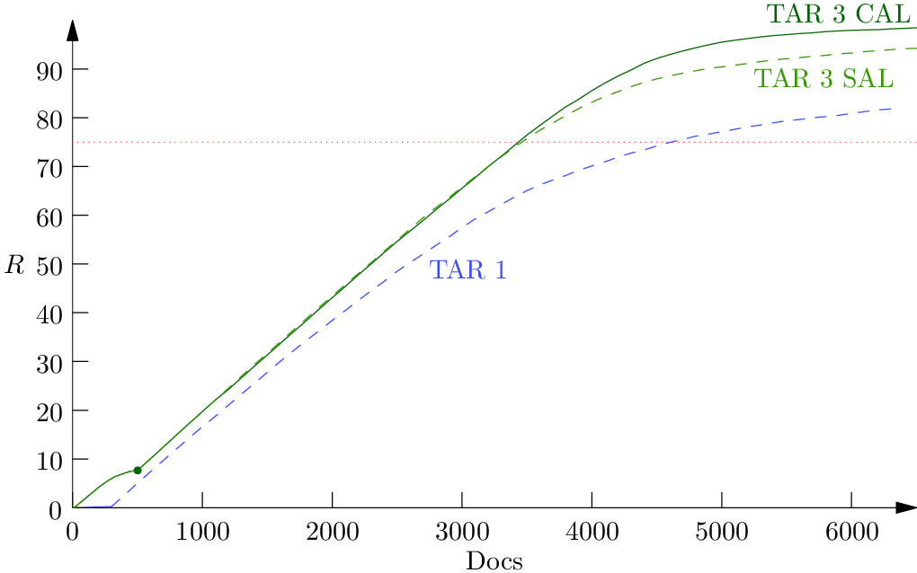
If you like graphs, the gain curves for all seven tasks are shown below.  Documents used for training are represented by solid lines, and documents not used for training are shown as dashed lines.  Dashed lines represent documents that could be produced without review if that is appropriate for the case.  A green dot is placed at the end of the review of cluster centers–this is the point where the TAR 3.0 SAL and TAR 3.0 CAL curves diverge, but sometimes they are so close together that it is hard to distinguish them without the dot.  Note that review of documents for control sets is not reflected in the gain curves, so the TAR 1.0 results require more document review than is implied by the curves.