Tag Archives: recall

Misleading Metrics and Irrelevant Research (Accuracy and F1)

If one algorithm achieved 98.2% accuracy while another had 98.6% for the same task, would you be surprised to find that the first algorithm required ten times as much document review to reach 75% recall compared to the second algorithm?  This article explains why some performance metrics don’t give an accurate view of performance for ediscovery purposes, and why that makes a lot of research utilizing such metrics irrelevant for ediscovery.

The key performance metrics for ediscovery are precision and recall.  Recall, R, is the percentage of all relevant documents that have been found.  High recall is critical to defensibility.  Precision, P, is the percentage of documents predicted to be relevant that actually are relevant.  High precision is desirable to avoid wasting time reviewing non-relevant documents (if documents will be reviewed to confirm relevance and check for privilege before production).  In other words, precision is related to cost.  Specifically, 1/P is the average number of documents you’ll have to review per relevant document found.  When using technology-assisted review (predictive coding), documents can be sorted by relevance score and you can choose any point in the sorted list and compute the recall and precision that would be achieved by treating documents above that point as being predicted to be relevant.  One can plot a precision-recall curve by doing precision and recall calculations at various points in the sorted document list.
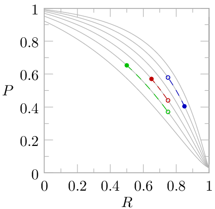
The precision-recall curve to the rightknn_precision compares two different classification algorithms applied to the same task.  To do a sensible comparison, we should compare precision values at the same level of recall.  In other words, we should compare the cost of reaching equally good (same recall) productions.  Furthermore, the recall level where the algorithms are compared should be one that is sensible for for ediscovery — achieving high precision at a recall level a court wouldn’t accept isn’t very useful.  If we compare the two algorithms at R=75%, 1-NN has P=6.6% and 40-NN has P=70.4%.  In other words, if you sort by relevance score with the two algorithms and review documents from top down until 75% of the relevant documents are found, you would review 15.2 documents per relevant document found with 1-NN and 1.4 documents per relevant document found with 40-NN.  The 1-NN algorithm would require over ten times as much document review as 40-NN.  1-NN has been used in some popular TAR systems.  I explained why it performs so badly in a previous article.

There are many other performance metrics, but they can be written as a mixture of precision and recall (see Chapter 7 of the current draft of my book).  Anything that is a mixture of precision and recall should raise an eyebrow — how can you mix together two fundamentally different things (defensibility and cost) into a single number and get a useful result?  Such metrics imply a trade-off between defensibility and cost that is not based on reality.  Research papers that aren’t focused on ediscovery often use such performance measures and compare algorithms without worrying about whether they are achieving the same recall, or whether the recall is high enough to be considered sufficient for ediscovery.  Thus, many conclusions about algorithm effectiveness simply aren’t applicable for ediscovery because they aren’t based on relevant metrics.
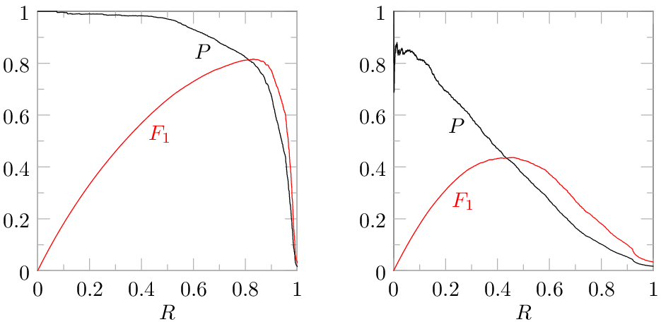
One popular metric is accuracy, knn_accuracywhich is the percentage of predictions that are correct.  If a system predicts that none of the documents are relevant and prevalence is 10% (meaning 10% of the documents are relevant), it will have 90% accuracy because its predictions were correct for all of the non-relevant documents.  If prevalence is 1%, a system that predicts none of the documents are relevant achieves 99% accuracy.  Such incredibly high numbers for algorithms that fail to find anything!  When prevalence is low, as it often is in ediscovery, accuracy makes everything look like it performs well, including algorithms like 1-NN that can be a disaster at high recall.  The graph to the right shows the accuracy-recall curve that corresponds to the earlier precision-recall curve (prevalence is 2.633% in this case), showing that it is easy to achieve high accuracy with a poor algorithm by evaluating it at a low recall level that would not be acceptable for ediscovery.  The maximum accuracy achieved by 1-NN in this case was 98.2% and the max for 40-NN was 98.6%.  In case you are curious, the relationship between accuracy, precision, and recall is:
ACC = 1 - \rho (1 - R) - \rho R (1 - P) / P
where \rho is the prevalence.

Another popular metric is the F1 score.knn_f1  I’ve criticized its use in ediscovery before.  The relationship to precision and recall is:
F_1 = 2 P R / (P + R)
The F1 score lies between the precision and the recall, and is closer to the smaller of the two.  As far as F1 is concerned, 30% recall with 90% precision is just as good as 90% recall with 30% precision (both give F1 = 0.45) even though the former probably wouldn’t be accepted by a court and the latter would.   F1 cannot be large at small recall, unlike accuracy, but it can be moderately high at modest recall, making it possible to achieve a decent F1 score even if performance is disastrously bad at the high recall levels demanded by ediscovery.  The graph to the right shows that 1-NN manages to achieve a maximum F1 of 0.64, which seems pretty good compared to the 0.73 achieved by 40-NN, giving no hint that 1-NN requires ten times as much review to achieve 75% recall in this example.

Hopefully this article has convinced you that it is important for research papers to use the right metric, specifically precision (or review effort) at high recall, when making algorithm comparisons that are useful for ediscovery.

TAR vs. Keyword Search Challenge, Round 3

This iteration of the challenge, held at the Education Hub at ILTACON 2018, was structured somewhat differently from round 1 and round 2 to give the audience a better chance of beating TAR.  Instead of submitting search queries on paper, participants submitted them through a web form using their phones, which allowed them to repeatedly tweak their queries and resubmit them.  I executed the queries in front of the participants, so they could see the exact recall achieved (since all documents were marked as relevant or non-relevant by a human reviewer in advance) almost instantaneously and they could utilize the performance information for their queries and the queries of other participants to guide improvements to their queries. This actually gave the participants an advantage over what they would experience in a real e-discovery project since performance measurements would normally require human evaluation of a random sample from the search output, which would make execution of several iterations of a query guided by performance evaluations very expensive in terms of review labor.  The audience got those performance evaluations for free even though the goal was to compare recall achieved for equal amounts of document review effort.  On the other hand, the audience did still have the disadvantages of having limited time and no familiarity with the documents.

As before, recall was evaluated for the top 3000 and top 6000 documents, which was enough to achieve high recall with TAR (even with the training documents included, so total review effort for TAR and the search queries was the same).  Audience members were free to work on any of the three topics that were used in previous versions of the challenge: law, medical industry, or biology.  Unfortunately, the audience was much smaller than previous versions of the challenge, and nobody chose to submit a query for the biology topic.

Previously, the TAR results were achieved by using the TAR 3.0 workflow to train with 200 cluster centers, documents were sorted based on the resulting relevance scores, and top-scoring documents were reviewed until the desired amount of review effort was expended without allowing predictions to be updated during that review (e.g., review of 200 training docs plus 2,800 top scoring docs to get the “Top 3,000” result).  I’ll call this TAR 3.0 SAL (SAL = Simple Active Learning, meaning the system is not allowed to learn during the review of top-scoring documents).  In practice you wouldn’t do that.  If you were reviewing top-scoring documents, you would allow the system to continue learning (CAL).  You would use SAL only if you were producing top-scoring documents without reviewing them since allowing learning to continue during the review would reduce the amount of review needed to achieve a desired level of recall.  I used TAR 3.0 SAL in previous iterations because I wanted to simulate the full review in front of the audience in a few seconds and TAR 3.0 CAL would have been slower.  This time, I did the TAR calculations in advance and present both the SAL and CAL results so you can see how much difference the additional learning from CAL made.

One other difference compared to previous versions of the challenge is how I’ve labeled the queries below.  This time, the number indicates which participant submitted the query and the letter indicates which one of his/her queries are being analyzed (if the person submitted more than one) rather than indicating a tweaking of the query that I added to try to improve the result.  In other words, all variations were tweaks done by the audience instead of by me.  Discussion of the results follows the tables, graphs, and queries below.

Recall
Medical Industry Top 3,000 Top 6,000
1a 3.0%
1b 17.4%
TAR 3.0 SAL 67.3% 83.7%
TAR 3.0 CAL 80.7% 88.5%


Recall
Law Top 3,000 Top 6,000
2 1.0%
3a 36.1% 42.3%
3b 45.3% 60.1%
3c 47.2% 62.6%
4 11.6% 13.8%
TAR 3.0 SAL 63.5% 82.3%
TAR 3.0 CAL 77.8% 87.8%

tar_vs_search3_medical

tar_vs_search3_law


1a)  Hospital AND New AND therapies
1b)  Hospital AND New AND (physicians OR doctors)
2)   Copyright AND mickey AND mouse
3a)  Schedule OR Amendments OR Trial OR Jury OR Judge OR Circuit OR Courtroom OR Judgement
3b)  Amendments OR Trial OR Jury OR Judge OR Circuit OR Courtroom OR Judgement OR trial OR law OR Patent OR legal
3c)  Amendments OR Trial OR Jury OR Judge OR Circuit OR Courtroom OR Judgement OR trial OR law OR Patent OR legal OR Plaintiff OR Defendant
4)  Privacy OR (Personally AND Identifiable AND Information) OR PII OR (Protected AND Speech)

TAR won across the board, as in previous iterations of the challenge.  Only one person submitted queries for the medical industry topic.  His/her revised query did a better job of finding relevant documents, but still returned fewer than 3,000 documents and fared far worse than TAR — the query was just not broad enough to achieve high recall.  Three people submitted queries on the law topic.  One of those people revised the query a few times and got decent results (shown in green), but still fell far short of the TAR result, with review of 6,000 documents from the best query finding fewer relevant documents than review of half as many documents with TAR 3.0 SAL (TAR 3.0 CAL did even better).  It is unfortunate that the audience was so small, since a larger audience might have done better by learning from each other’s submissions.  Hopefully I’ll be able to do this with a bigger audience in the future.

TAR, Proportionality, and Bad Algorithms (1-NN)

Should proportionality arguments allow producing parties to get away with poor productions simply because they wasted a lot of effort due to an extremely bad algorithm?  This article examines one such bad algorithm that has been used in major review platforms, and shows that it could be made vastly more effective with a very minor tweak.  Are lawyers who use platforms lacking the tweak committing malpractice by doing so?

Last year I was moderating a panel on TAR (predictive coding) and I asked the audience what recall level they normally aim for when using TAR.  An attendee responded that it was a bad question because proportionality only required a reasonable effort.  Much of the audience expressed agreement.  This should concern everyone.  If quality of result (e.g., achieving a certain level of recall) is the goal, the requesting party really has no business asking how the result was achieved–any effort wasted by choosing a bad algorithm is born by the producing party.  On the other hand, if the target is expenditure of a certain amount of effort, doesn’t the requesting party have the right to know and object if the producing party has chosen a methodology that is extremely inefficient?

The algorithm I’ll be picking on today is a classifier called 1-nearest neighbor, or 1-NN.  You may be using it without ever having heard that name, so pay attention to my description of it and see if it sounds familiar.  To predict whether a document is relevant, 1-NN finds the single most similar training document and predicts the relevance of the unreviewed document to be the same.  If a relevance score is desired instead of a yes/no relevance prediction, the relevance score can be taken to be the similarity value if the most similar training document is relevant, and it can be taken to be the negative of the similarity value if the most similar training document is non-relevant.  Here is a precision-recall curve for the 1-NN algorithm used in a TAR 1.0 workflow trained with randomly-selected documents:

knn_1

The precision falls off a cliff above 60% recall.  This is not due to inadequate training–the cliff shown above will not go away no matter how much training data you add.  To understand the implications, realize that if you sort the documents by relevance score and review from the top down until you reach the desired level of recall, 1/P at that recall tells the average number of documents you’ll review for each relevant document you find.  At 60% recall, precision is 67%, so you’ll review 1.5 documents (1/0.67 = 1.5) for each relevant document you find.  There is some effort wasted in reviewing those 0.5 non-relevant documents for each relevant document you find, but it’s not too bad.  If you keep reviewing documents until you reach 70% recall, things get much worse.  Precision drops to about 8%, so you’ll encounter so many non-relevant documents after you get past 60% recall that you’ll end up reviewing 12.5 documents for each relevant document you find.  You would surely be tempted to argue that proportionality says you should be able to stop at 60% recall because the small gain in result quality of going from 60% recall to 70% recall would cost nearly ten times as much review effort.  But does it really have to be so hard to get to 70% recall?

It’s very easy to come up with an algorithm that can reach higher recall without so much review effort once you understand why the performance cliff occurs.  When you sort the documents by relevance score with 1-NN, the documents where the most similar training document is relevant will be at the top of the list.  The performance cliff occurs when you start digging into the documents where the most similar training document is non-relevant.  The 1-NN classifier does a terrible job of determining which of those documents has the best chance of being relevant because it ignores valuable information that is available.  Consider two documents, X and Y, that both have a non-relevant training document as the most similar training document, but document X has a relevant training document as the second most similar training document and document Y has a non-relevant training document as the second most similar.  We would expect X to have a better chance of being relevant than Y, all else being equal, but 1-NN cannot distinguish between the two because it pays no attention to the second most similar training document.  Here is the result for 2-NN, which takes the two most similar training document into account:

knn_2

Notice that 2-NN easily reaches 70% recall (1/P is 1.6 instead of 12.5), but it does have a performance cliff of its own at a higher level of recall because it fails to make use of information about the third most similar training document.  If we utilize information about the 40 most similar training documents we get much better performance as shown by the solid lines here:

knn_40

It was the presence of non-relevant training documents that tripped up the 1-NN algorithm because the non-relevant training document effectively hid the existence of evidence (similar training documents that were relevant) that a document might be relevant, so you might think the performance cliff could be avoided by omitting non-relevant documents from the training.  The result of doing that is shown with dashed lines in the figure above.  Omitting non-relevant training documents does help 1-NN at high recall, though it is still far worse than 40-NN with the non-relevant training documents include (omitting the non-relevant training documents actually harms 40-NN, as shown by the red dashed line).  A workflow that focuses on reviewing documents that are likely to be relevant, such as TAR 2.0, rather than training with random documents, will be less impacted by 1-NN’s shortcomings, but why would you ever suffer the poor performance of 1-NN when 40-NN requires such a minimal modification of the algorithm?

You might wonder whether the performance cliff shown above is just an anomaly.  Here are precision-recall curves for several additional categorization tasks with 1-NN on the left and 40-NN on the right.

1nn_vs_40nn_several_tasks

Sometimes the 1-NN performance cliff occurs at high enough recall to allow a decent production, but sometimes it keeps you from finding even half of the relevant documents.  Should a court accept less than 50% recall when the most trivial tweak to the algorithm could have achieved much higher recall with roughly the same amount of document review?

Of course, there are many factors beyond the quality of the classifier, such as the choice of TAR 1.0 (SPL and SAL), TAR 2.0 (CAL), or TAR 3.0 workflows, that impact the efficiency of the process.  The research by Grossman and Cormack that courts have relied upon to justify the use of TAR because it reaches recall that is comparable to or better than an exhaustive human review is based on CAL (TAR 2.0) with good classifiers, whereas some popular software uses TAR 1.0 (less efficient if documents will be reviewed before production) and poor classifiers such as 1-NN.  If the producing party vows to reach high recall and bears the cost of choosing bad software and/or processes to achieve that, there isn’t much for the requesting party to complain about  (though the producing party could have a bone to pick with an attorney or service provider who recommended an inefficient approach). On the other hand, if the producing party argues that low recall should be tolerated because decent recall would require too much effort, it seems that asking whether the algorithms used are unnecessarily inefficient would be appropriate.

TAR vs. Keyword Search Challenge, Round 2

During my presentation at the South Central eDiscovery & IG Retreat I challenged the audience to create keyword searches that would work better than technology-assisted review (predictive coding).  This is similar to the experiment done a few months earlier.  See this article for more details.  The audience again worked in groups to construct keyword searches for two topics.  One topic, articles on law, was the same as last time.  The other topic, the medical industry, was new (it replaced biology).

Performance was evaluated by comparing the recall achieved for equal amounts of document review effort (the population was fully categorized in advance, so measurements are exact, not estimates).  Recall for the top 3000 keyword search matches was compared to recall from reviewing 202 training documents (2 seed documents plus 200 cluster centers using the TAR 3.0 method) and 2798 documents having the highest relevance scores from TAR.  Similarly, recall from the top 6000 keyword search matches was compared to recall from review of 6000 documents with TAR.  Recall from all documents matching a search query was also measured to find the maximum recall that could be achieved with the query.

The search queries are shown after the performance tables and graphs.  When there is an “a” and “b” version of the query, the “a” version was the audience’s query as-is, and the “b” query was tweaked by me to remove restrictions that were limiting the number of relevant documents that could be found.  The results are discussed at the end of the article.

Medical Industry Recall
Query Total Matches Top 3,000 Top 6,000 All
1a 1,618 14.4% 14.4%
1b 3,882 32.4% 40.6% 40.6%
2 7,684 30.3% 42.2% 46.6%
3a 1,714 22.4% 22.4%
3b 16,756 32.7% 44.6% 71.1%
4a 33,925 15.3% 20.3% 35.2%
4b 58,510 27.9% 40.6% 94.5%
TAR 67.3% 83.7%


Law Recall
Query Total Matches Top 3,000 Top 6,000 All
5 36,245 38.8% 56.4% 92.3%
6 25,370 51.9% 72.4% 95.7%
TAR 63.5% 82.3%

tar_vs_search2_medical

tar_vs_search2_law


1a) medical AND (industry OR business) AND NOT (scientific OR research)
1b) medical AND (industry OR business)
2) (revenue OR finance OR market OR brand OR sales) AND (hospital OR health OR medical OR clinical)
3a) (medical OR hospital OR doctor) AND (HIPPA OR insurance)
3b) medical OR hospital OR doctor OR HIPPA OR insurance
4a) (earnings OR profits OR management OR executive OR recall OR (board AND directors) OR healthcare OR medical OR health OR hospital OR physician OR nurse OR marketing OR pharma OR report OR GlaxoSmithKline OR (united AND health) OR AstraZeneca OR Gilead OR Sanofi OR financial OR malpractice OR (annual AND report) OR provider OR HMO OR PPO OR telemedicine) AND NOT (study OR research OR academic)
4b) earnings OR profits OR management OR executive OR recall OR (board AND directors) OR healthcare OR medical OR health OR hospital OR physician OR nurse OR marketing OR pharma OR report OR GlaxoSmithKline OR (united AND health) OR AstraZeneca OR Gilead OR Sanofi OR financial OR malpractice OR (annual AND report) OR provider OR HMO OR PPO OR telemedicine
5) FRCP OR Fed OR litigation OR appeal OR immigration OR ordinance OR legal OR law OR enact OR code OR statute OR subsection OR regulation OR rules OR precedent OR (applicable AND law) OR ruling
6) judge OR (supreme AND court) OR court OR legislation OR legal OR lawyer OR judicial OR law OR attorney

As before, TAR won across the board, but there were some surprises this time.

For the medical industry topic, review of 3000 documents with TAR achieved higher recall than any keyword search achieved with review of 6000 documents, very similar to results from a few months ago.  When all documents matching the medical industry search queries were analyzed, two queries did achieve high recall (3b and 4b, which are queries I tweaked to achieve higher recall), but they did so by retrieving a substantial percentage of the 100,000 document population (16,756 and 58,510 documents respectively).  TAR can reach any level of recall by simply taking enough documents from the sorted list—TAR doesn’t run out of matches like a keyword search does.  TAR matches the 94.6% recall that query 4b achieved (requiring review of 58,510 documents) with review of only 15,500 documents.

Results for the law topic were more interesting.  The two queries submitted for the law topic both performed better than any of the queries submitted for that topic a few months ago.  Query 6 gave the best results, with TAR beating it by only a modest amount.  If all 25,370 documents matching query 6 were reviewed, 95.7% recall would be achieved, which TAR could accomplish with review of 24,000 documents.  It is worth noting that TAR 2.0 would be more efficient, especially at very high recall.  TAR 3.0 gives the option to produce documents without review (not utilized for this exercise), plus computations are much faster due to there being vastly fewer training documents, which is handy for simulating a full review live in front of an audience in a few seconds.

TAR vs. Keyword Search Challenge

During my presentation at the NorCal eDiscovery & IG Retreat I challenged the audience to create keyword searches that would work better than technology-assisted review (predictive coding) for two topics.  Half of the room was tasked with finding articles about biology (science-oriented articles, excluding medical treatment) and the other half searched for articles about current law (excluding proposed laws or politics).  I ran one of the searches against TAR in Clustify live during the presentation (Clustify’s “shadow tags” feature allows a full document review to be simulated in a few minutes using documents that were pre-categorized by human reviewers), but couldn’t do the rest due to time constraints.  This article presents the results for all the queries submitted by the audience.

The audience had limited time to construct queries (working together in groups), they weren’t familiar with the data set, and they couldn’t do sampling to tune their queries, so I’m not claiming the exercise was comparable to an e-discovery project.  Still, it was entertaining.  The topics are pretty simple, so a large percentage of the relevant documents can be found with a pretty simple search using some broad terms.  For example, a search for “biology” would find 37% of the biology documents.  A search for “law” would find 71% of the law articles.  The trick is to find the relevant documents without pulling in too many of the non-relevant ones.

To evaluate the results, I measured the recall (percentage of relevant documents found) from the top 3,000 and top 6,000 hits on the search query (3% and 6% of the population respectively).  I’ve also included the recall achieved by looking at all docs that matched the search query, just to see what recall the search queries could achieve if you didn’t worry about pulling in a ton of non-relevant docs.  For the TAR results I used TAR 3.0 trained with two seed documents (one relevant from a keyword search and one random non-relevant document) followed by 20 iterations of 10 top-scoring cluster centers, so a total of 202 training documents (no control set needed with TAR 3.0).  To compare to the top 3,000 search query matches, the 202 training documents plus 2,798 top-scoring documents were used for TAR, so the total document review (including training) would be the same for TAR and the search query.

The search engine in Clustify is intended to help the user find a few seed documents to get active learning started, so it has some limitations.  If the audience’s search query included phrases, they were converted an AND search enclosed in parenthesis.  If the audience’s query included a wildcard, I converted it to a parenthesized OR search by looking at the matching words in the index and selecting only the ones that made sense (i.e., I made the queries better than they would have been with an actual wildcard).  I noticed that there were a lot of irrelevant words that matched the wildcards.  For example, “cell*” in a biology search should match cellphone, cellular, cellar, cellist, etc., but I excluded such words.  I would highly recommend that people using keyword search check to see what their wildcards are actually matching–you may be pulling in a lot of irrelevant words.  I removed a few words from the queries that weren’t in the index (so the words shown all actually had an impact).  When there is an “a” and “b” version of the query, the “a” version was the audience’s query as-is, and the “b” query was tweaked by me to retrieve more documents.

The tables below show the results.  The actual queries are displayed below the tables.  Discussion of the results is at the end.

Biology Recall
Query Total Matches Top 3,000 Top 6,000 All Matches
1 4,407 34.0% 47.2% 47.2%
2 13,799 37.3% 46.0% 80.9%
3 25,168 44.3% 60.9% 87.8%
4a 42 0.5% 0.5%
4b 2,283 20.9% 20.9%
TAR 72.1% 91.0%
Law Recall
Query Total Matches Top 3,000 Top 6,000 All Matches
5a 2,914 35.8% 35.8%
5b 9,035 37.2% 49.3% 60.6%
6 534 2.9% 2.9%
7 27,288 32.3% 47.1% 79.1%
TAR 62.3% 80.4%

tar_vs_search_biology

tar_vs_search_law

1) organism OR microorganism OR species OR DNA

2) habitat OR ecology OR marine OR ecosystem OR biology OR cell OR organism OR species OR photosynthesis OR pollination OR gene OR genetic OR genome AND NOT (treatment OR generic OR prognosis OR placebo OR diagnosis OR FDA OR medical OR medicine OR medication OR medications OR medicines OR medicated OR medicinal OR physician)

3) biology OR plant OR (phyllis OR phylos OR phylogenetic OR phylogeny OR phyllo OR phylis OR phylloxera) OR animal OR (cell OR cells OR celled OR cellomics OR celltiter) OR (circulation OR circulatory) OR (neural OR neuron OR neurotransmitter OR neurotransmitters OR neurological OR neurons OR neurotoxic OR neurobiology OR neuromuscular OR neuroscience OR neurotransmission OR neuropathy OR neurologically OR neuroanatomy OR neuroimaging OR neuronal OR neurosciences OR neuroendocrine OR neurofeedback OR neuroscientist OR neuroscientists OR neurobiologist OR neurochemical OR neuromorphic OR neurohormones OR neuroscientific OR neurovascular OR neurohormonal OR neurotechnology OR neurobiologists OR neurogenetics OR neuropeptide OR neuroreceptors) OR enzyme OR blood OR nerve OR brain OR kidney OR (muscle OR muscles) OR dna OR rna OR species OR mitochondria

4a) statistically AND ((laboratory AND test) OR species OR (genetic AND marker) OR enzyme) AND NOT (diagnosis OR treatment OR prognosis)

4b)  (species OR (genetic AND marker) OR enzyme) AND NOT (diagnosis OR treatment OR prognosis)

5a) federal AND (ruling OR judge OR justice OR (appellate OR appellant))

5b) ruling OR judge OR justice OR (appellate OR appellant)

6) amendments OR FRE OR whistleblower

7) ((law OR laws OR lawyer OR lawyers OR lawsuit OR lawsuits OR lawyering) OR (regulation OR regulations) OR (statute OR statutes) OR (standards)) AND NOT pending

TAR beat keyword search across the board for both tasks.  The top 3,000 documents returned by TAR achieved higher recall than the top 6,000 documents for any keyword search.  In other words, if documents will be reviewed before production, TAR achieves better results (higher recall) with half as much document review compared to any of the keyword searches.  The top 6,000 documents returned by TAR achieved higher recall than all of the documents matching any individual keyword search, even when the keyword search returned 27,000 documents.

Similar experiments were performed later with many similarities but also some notable differences in the structure of the challenge and the results.  You can read about them here: round 2, round 3, round 4, round 5, and round 6.

Substantial Reduction in Review Effort Required to Demonstrate Adequate Recall

Measuring the recall achieved to within +/- 5% to demonstrate that a production is defensible can require reviewing a substantial number of random documents.  For a case of modest size, the amount of review required to measure recall can be larger than the amount of review required to actually find the responsive documents with predictive coding.  This article describes a new method requiring much less document review to demonstrate that adequate recall has been achieved.  This is a brief overview of a more detailed paper I’ll be presenting at the DESI VII Workshop on June 12th (slides available here).

The proportion of a population having some property can be estimated to within +/- 5% by measuring the proportion on a random sample of 400 documents (you’ll also see the number 385 being used, but using 400 will make it easier to follow the examples).  To measure recall we need to know what proportion of responsive documents are produced, so we need a sample of 400 random responsive documents.  Since we don’t know which documents in the population are responsive, we have to select documents randomly and review them until 400 responsive ones are found.  If prevalence is 10% (10% of the population is responsive), that means reviewing roughly 4,000 documents to find 400 that are relevant so that recall can be estimated.  If prevalence is 1%, it means reviewing roughly 40,000 random documents to measure recall.  This can be quite a burden.

multistage_acceptance_from_multistageOnce recall is measured, a decision must be made about whether it is high enough.  Suppose you decide that if at least 300 of the 400 random responsive documents were produced (75%) the production is acceptable.  For any actual level of recall, the probability of accepting the production can be computed (see figure to right).  The probability of accepting a production where the actual recall is less than 70% will be very low, and the probability of rejecting a production where the actual recall is greater than 80% will also be low — this comes from the fact that a sample of 400 responsive documents is sufficient to measure recall to within +/- 5%.

multistage_acceptance_procedureThe idea behind the new method is to achieve the same probability profile for accepting/rejecting a production using a multi-stage acceptance test.  The multi-stage test gives the possibility of stopping the process and declaring the production accepted/rejected long before reviewing 400 random responsive documents.  The procedure is shown in the flowchart to the right (click to enlarge).  A decision may be reached after reviewing enough documents to find just 25 random documents that are responsive.  If a decision isn’t made after reviewing 25 responsive documents, review continues until 50 responsive documents are found and another test is applied.  At worst, documents will be reviewed until 400 responsive documents are found (the same as the traditional direct recall estimation method).

multistage_barriers_85_recall_pathsThe figure to the right shows six examples of the multi-stage acceptance test being applied when the actual recall is 85%.  Since 85% is well above the 80% upper bound of the 75% +/- 5% range, we expect this production to virtually always be accepted.  The figure shows that acceptance can occur long before reviewing a full 400 random responsive documents.  The number of random responsive documents reviewed is shown on the vertical axis.  Toward the bottom of the graph the sample is very small and the percentage of the sample that has been produced may deviate greatly from the right answer of 85%.  As you go up the sample gets larger and the proportion of the sample that is produced is expected to get closer to 85%.  When a green decision boundary is touched, causing the production to be accepted as having sufficiently high recall, the color of the remainder of the path is changed to yellow — the yellow part represents the document review that is avoided by using the multi-stage acceptance method (since the traditional direct recall measurement would involve going all the way to 400 responsive documents).  As you can see, when the actual recall is 85% the number of random responsive documents that must be reviewed is often 50 or 100, not 400.

multistage_effort_for_multistageThe figure to the right shows the average number of documents that must be reviewed using the multi-stage acceptance procedure from the earlier flowchart.  The amount of review required can be much less than 400 random responsive documents.  In fact, the further above/below the 75% target (called the “splitting recall” in the paper) the actual recall is, the less document review is required (on average) to come to a conclusion about whether the production’s recall is high enough.  This creates an incentive for the producing party to aim for recall that is well above the minimum acceptable level since it will be rewarded with a reduced amount of document review to confirm the result is adequate.

It is important to note that the multi-stage procedure provides an accept/reject result, not a recall estimate.  If you follow the procedure until an accept/reject boundary is hit and then use the proportion of the sample that was produced as a recall estimate, that estimate will be biased (the use of “unbiased” in the paper title refers to the sampling being done on the full population, not on a subset [such as the discard set] that would cause a bias due to inconsistency in review of different subsets).

You may want to use a splitting recall other than 75% for the accept/reject decision — the full paper provides tables of values necessary for doing that.

Webinar: 10 Years Forward and Back: Automation in eDiscovery

George Socha, Doug Austin, David Horrigan, Bill Dimm, and Bill Speros will give presentations in this webinar on the history and future of ediscovery moderated by Mary Mack on December 1, 2016.  Bill Dimm will talk about the evolution of predictive coding technologies and our understanding of best practices, including recall estimation, the evil F1 score, research efforts, pre-culling, and the TAR 1.0, 2.0, and 3.0 workflows.  CLICK HERE FOR RECORDING OF WEBINAR, SLIDES, AND LINKS TO RELATED RESOURCES.

Gain Curves

You may already be familiar with the precision-recall curve, which describes the performance of a predictive coding system.  Unfortunately, the precision-recall curve doesn’t (normally) display any information about the cost of training the system, so it isn’t convenient when you want to compare the effectiveness of different training methodologies.  This article looks at the gain curve, which is better suited for that purpose.

The gain curve shows how the recall achieved depends on the number of documents reviewed (slight caveat to that at the end of the article).  Recall is the percentage of all relevant documents that have been found.  High recall is important for defensibility.  Here is an example of a gain curve (click to enlarge):

gain_curve_single

The first 12,000 documents reviewed in this example are randomly selected documents used to train the system.  Prevalence is very low in this case (0.32%), so finding relevant documents using random selection is hard.  The system needs to be exposed to a large enough number of relevant training documents for it to learn what they look like so it can make good predictions for the relevance of the remaining documents.

After the 12,000 training documents are reviewed the system orders the remaining documents to put the ones that are most likely to be relevant (based on patterns detected during training) at the top of the list.  To distinguish the training phase from the review phase I’ve shown the training phase as a solid line and review phase as a dashed line.  Review of the remaining documents starts at the top of the sorted list.  The gain curve is very steep at the beginning of the review phase because most of the documents being reviewed are relevant, so they have a big impact on recall.  As the review progresses the gain curve becomes less steep because you end up reviewing documents that are less likely to be relevant.  Review proceeds until a desired level of recall, such as 75% (the horizontal dotted line), is achieved.  The goal is to find the system and workflow that achieves the recall target at the lowest cost (i.e., the one that crosses the dotted line farthest to the left, with some caveats below).

What is the impact of using the same system with a larger or smaller number of randomly selected training documents?  This figure shows the gain curves for 9,000 and 15,000 training documents in addition to the 12,000 training document curve seen earlier:

gain_curve_multi

If the goal is to reach 75% recall, 12,000 is the most efficient option among the three considered because it crosses the horizontal dotted line with the least document review.  If the target was a lower level of recall, such as 70%, 9,000 training documents would be a better choice.  A larger number of training documents usually leads to better predictions (the gain curve stays steep longer during the review phase), but there is a point where the improvement in the predictions isn’t worth the cost of reviewing additional training documents.

The discussion above assumed that the cost of reviewing a document during the training phase is the same as the cost of reviewing a document during the review phase.  That will not be the case if expensive subject matter experts are used to review the training documents and low-cost contract reviewers are used for the review phase.  In that situation, the optimal result is less straightforward to identify from the gain curve.

In some situations it may be possible produce documents without reviewing them if there is no concern about disclosing privileged documents (because there are none or because they are expected to be easy to identify by looking at things like the sender/recipient email address) or non-relevant documents (because there is no concern about them containing trade secrets or evidence of bad acts not covered by the current litigation).  When it is okay to produce documents without reviewing them, the document review associated with the dashed part of the curve can be eliminated in whole or in part.  For example, documents predicted to be relevant with high confidence may be produced without review (unless they are identified as potential privileged), whereas documents with a lower likelihood of being relevant might be reviewed to avoid disclosing too many non-relevant documents.  Again, the gain curve would not show the optimal choice in a direct way–you would need to balance the potential harm (even if small) of producing non-relevant documents against the cost of additional training.

The predictive coding process described in this article, random training documents followed by review (with no additional learning by the algorithm), is sometimes known as Simple Passive Learning (SPL), which is one example of a TAR 1.0 workflow.  To determine the optimal point to switch from training to review with TAR 1.0, a random set of documents known as a control set is reviewed and used to monitor learning progress by comparing the predictions for the control set documents to their actual relevance tags.  Other workflows and analysis of their efficiency via gain curves will be the subject of my next article.

Using Extrapolated Precision for Performance Measurement

This is a brief overview of my paper “Information Retrieval Performance Measurement Using Extrapolated Precision,” which I’ll be presenting on June 8th at the DESI VI workshop at ICAIL 2015 (slides now available here).  The paper provides a novel method for extrapolating a precision-recall point to a different level of recall, and advocates making performance comparisons by extrapolating results for all systems to the same level of recall if the systems cannot be evaluated at exactly the same recall (e.g., some predictive coding systems produce a binary yes/no prediction instead of a relevance score, so the user cannot select the recall that will be achieved).

High recall (finding most of the relevant documents) is important in e-discovery for defensibility.  High precision is desirable to ensure that there aren’t a lot of non-relevant documents mixed in with the relevant ones (i.e., high precision reduces the cost of review for responsiveness and privilege).  Making judgments about the relative performance of two predictive coding systems knowing only a single precision-recall point for each system is problematic—if one system has higher recall but lower precision for a particular task, is it the better system for that task?

There are various performance measures like the F1 score that combine precision and recall into a single number to allow performance comparisons.  Unfortunately, such measures often assume a trade-off between precision and recall that is not appropriate for e-discovery (I’ve written about problems with the  F1 score before).  To understand the problem, it is useful to look at how F1 varies as a function of the recall where it is measured.  Here are two precision-recall curves, with the one on the left being for an easy categorization task and the one on the right being for a hard task, with the F1 score corresponding to each point on the precision-recall curve superimposed:

f1_compare2If we pick a single point from the precision-recall curve and compute the value of F1 for that point, the resulting F1 is very sensitive to the precision-recall point we choose.  F1 is maximized at 46% recall in the graph on the right, which means that the trade-off between precision and recall that F1 deems to be reasonable implies that it is not worthwhile to produce more than 46% of the relevant documents for that task because precision suffers too much when you push to higher recall.  That is simply not compatible with the needs of e-discovery.  In e-discovery, the trade-off  between precision (cost) and recall required should be dictated by proportionality, not by some performance measure that is oblivious to the value of the case.  Other problems with the F1 score are detailed in the paper.

The strong dependence that F1 has on recall as we move along the precision-recall curve means that it is easy to draw wrong conclusions about which system is performing better when performance is measured at different levels of recall.  This strong dependence on recall occurs because the contours of equal F1 are not shaped like precision-recall curves, so a precision-recall curve will cut across many contours.   In order to have the freedom to measure performance at recall levels that are relevant for e-discovery (e.g., 75% or higher) without drawing wrong conclusions about which system is performing best, the paper proposes a performance measure that has constant-performance contours that are shaped like precision-recall curves, so the performance measure depends much less on the recall level where the measurement is made than F1 does. In other words, the proposed performance measure aims to be sensitive to how well the system is working while being insensitive to the specific point on the precision-recall curve where the measurement is made.  This graph compares the constant-performance contours for F1 to the measure proposed in the paper:

f1_x_contours

Since the constant-performance contours are shaped like typical precision-recall curves, we can view this measure as being equivalent to extrapolating the precision-recall point to some other target recall level, like 75%, by simply finding an idealized precision-recall curve that passes through the point and moving along that curve to the target recall.  This figure illustrates extrapolation of precision measurements for three different systems at different recall levels to 75% recall for comparison:

x_extrapolate

Finally, here is what the performance measure looks like if we evaluate it for each point in the two precision-recall curves from the first figure:

x_compare2

The blue performance curves are much flatter than the red F1 curves from the first figure, so the value is much less sensitive to the recall level where it is measured.  As an added bonus, the measure is an extrapolated estimate of the precision that the system would achieve at 75% recall, so it is inversely proportional to the cost of the document review needed (excluding training and testing) to reach 75% recall.  For more details, read the paper or attend my talk at DESI VI.

Can You Really Compete in TREC Retroactively?

I recently encountered a marketing piece where a vendor claimed that their tests showed their predictive coding software demonstrated favorable performance compared to the software tested in the 2009 TREC Legal Track for Topic 207 (finding Enron emails about fantasy football).  I spent some time puzzling about how they could possibly have measured their performance when they didn’t actually participate in TREC 2009.

One might question how meaningful it is to compare to performance results from 2009 since the TREC participants have probably improved their software over the past six years.  Still, how could you do the comparison if you wanted to?  The stumbling block is that TREC did not produce a yes/no relevance determination for all of the Enron emails.  Rather, they did stratified sampling and estimated recall and prevalence for the participating teams by producing relevance determinations for just a few thousand emails.

Stratified sampling means that the documents are separated into mutually-exclusive buckets called “strata.”  To the degree that stratification manages to put similar things into the same stratum, it can produce better statistical estimates (smaller uncertainty for a given amount of document review).  The TREC Legal Track for 2009 created a stratum containing documents that all participants agreed were relevant.  It also created four strata containing documents that all but one participant predicted were relevant (there were four participants, so one stratum for each dissenting participant).  There were six strata where two participants agreed on relevance, and four strata where only one of the four participants predicted the documents were relevant.  Finally, there was one stratum containing documents that all participants predicted were non-relevant, which was called the “All-N” stratum.  So, for each stratum a particular participant either predicted that all of the documents were relevant or they predicted that all of the documents were non-relevant.  You can view details about the strata in table 21 on page 39 here.  Here is an example of what a stratification might look like for just two participants (the number of documents shown and percentage that are relevant may differ from the actual data):

stratification

A random subset of documents from each stratum was chosen and reviewed so that the percentage of the documents in the stratum that were relevant could be estimated.  Multiplying that percentage by the number of documents in the stratum gives an estimate for the number of relevant documents in the stratum.  Combining the results for the various strata allows precision and recall estimates to be computed for each participant.  How could this be done for a team that didn’t participate?  Before presenting some ideas, it will be useful to have some notation:

N[i] = number of documents in stratum i
n[i] = num docs in i that were assessed by TREC
n+[i] = num docs in i that TREC assessed as relevant
V[i] = num docs in i that vendor predicted were relevant
v[i] = num docs in i that vendor predicted were relevant and were assessed by TREC
v+[i] = num docs in i that vendor predicted were relevant and assessed as relevant by TREC

sampling

To make some of the discussion below more concrete, I’ll provide formulas for computing the number of true positives (TP), false positives (FP), and false negatives (FN).  The recall and precision can then be computed from:

R = TP / (TP + FN)
P = TP / (TP + FP)

Here are some ideas I came up with:

1) They could have checked to see which strata the documents they predicted to be relevant fell into and applied the percentages TREC computed to their data.  The problem is that since they probably didn’t identify all of the documents in a stratum as being relevant the percentage of documents that were estimated to be relevant for the stratum by TREC wouldn’t really be applicable.  If their system worked really well, they may have only predicted that the truly relevant documents from the stratum were relevant.  If their system worked badly, their system may have predicted that only the truly non-relevant documents from the stratum were relevant.  This approach could give estimates that are systematically too low or too high.  Here are the relevant formulas (summing over strata, i):

TP = Sum{ V[i] * n+[i] / n[i] }
FP = Sum{ V[i] * (1 – n+[i]/n[i]) }
FN = Sum{ (N[i] – V[i]) * n+[i] / n[i] }

2) Instead of using the percentages computed by TREC, they could have computed their own percentages by looking at only the documents in the stratum that they predicted were relevant and were reviewed by TREC to give a relevance determination.  This would eliminate the possible bias from approach (1), but it also means that the percentages would be computed from a smaller sample, so the uncertainty in the percentage that are relevant would be bigger.  The vendor didn’t provide confidence intervals for their results.  Here is how the computation would go:

TP = Sum{ V[i] * v+[i] / v[i] }
FP = Sum{ V[i] * (1 – v+[i]/v[i]) }
FN = Sum{ (N[i] – V[i]) * (n+[i] – v+[i]) / (n[i] – v[i]) }

It’s possible that for some strata there would be no overlap between the documents TREC assessed and the documents the vendor predicted to be relevant since TREC typically assessed only about 4% of each stratum for Topic 207 (except the All-N stratum, where they assessed only 0.46%).  This approach wouldn’t work for those strata since v[i] would be 0.  For strata where v[i] is 0, one might use approach (1) and hope it isn’t too wrong.

3) A more sophisticated tweak on (2) would be to use the ratio n+[i]/n[i] from (1) to generate a Bayesian prior probability distribution for the proportion of documents predicted by the vendor to be relevant that actually are relevant, and then use v+[i] and v[i] to compute a posterior distribution for that proportion and use the mean of that distribution instead of v+[i]/v[i] in the computation. The idea is to have a smooth interpolation between using n+[i]/n[i] and using v+[i]/v[i] as the proportion of documents estimated to be relevant, where the interpolation would be closer to v+[i]/v[i] if v[i] is large (i.e., if there is enough data for v+[i]/v[i] to be reasonably accurate).  The result would be sensitive to choices made in creating the Bayesian prior (i.e., how much variance to give the probability distribution), however.

4) They could have ignored all of the documents that weren’t reviewed in TREC (over 500,000 of them) and just performed their predictions and analysis on the 3,709 documents that had relevance assessments (training documents should come from the set TREC didn’t assess and should be reviewed by the vendor to simulate actual training at TREC being done by the participants).  It would be very important to weight the results to compensate for the fact that those 3,709 documents didn’t all have the same probability of being selected for review.  TREC oversampled the documents that were predicted to be relevant compared to the remainder (i.e., the number of documents sampled from a stratum was not simply proportional to the number of documents in the stratum), which allowed their stratification scheme to do a good job of comparing the participating teams to each other at the expense of having large uncertainty for some quantities like the total number of relevant documents.  The prevalence of relevant documents in the full population was 1.5%, but 9.0% of the documents having relevance assessments were relevant.  Without weighting the results to compensate for the uneven sampling, you would be throwing away over half a million non-relevant documents without giving the system being tested the opportunity to incorrectly predict that some of them are relevant, which would lead to an inflated precision estimate.  The expression “shooting fish in a barrel” comes to mind.  Weighting would be accomplished by dividing by the probability of the document having been chosen (after this article was published I learned that this is called the Horvitz-Thompson estimator, and it is what the TREC evaluation toolkit uses), which is just n[i]/N[i], so the computation would be:

TP = Sum{ (N[i]/n[i]) * v+[i] }
FP = Sum{ (N[i]/n[i]) * (v[i] – v+[i]) }
FN = Sum{ (N[i]/n[i]) * (n+[i] – v+[i]) }

Note that if N[i]/n[i] is equal to V[i]/v[i], which is expected to be approximately true since the subset of a stratum chosen for assessment by TREC is random, the result would be equal to that from (2).  If N[i]/n[i] is not equal to V[i]/v[i] for a stratum, we would have the disturbing result that the estimate for TP+FP for that stratum would not equal the number of documents the vendor predicted to be relevant for that stratum, V[i].

5) The vendor could have ignored the TREC relevance determinations, simply doing their own.  That would be highly biased in the vendor’s favor because there would be a level of consistency between relevance determinations for the training data and testing data that did not exist for TREC participants.  At TREC the participants made their own relevance determinations to train their systems and a separate set of Topic Authorities made the final relevance judgments that determined the performance numbers.  To the degree that participants came to different conclusions about relevance compared to the Topic Authorities, their performance numbers would suffer.  A more subtle problem with this approach is that the vendor’s interpretation of the relevance criteria would inevitably be somewhat different from that of TREC assessors (studies have shown poor agreement between different review teams), which could make the classification task either easier or harder for a computer.  As an extreme example, if the vendor took all documents containing the word “football” to be relevant and all other documents to be non-relevant, it would be very easy for a predictive coding system to identify that pattern and achieve good performance numbers.

Approaches (1)-(4) would all give the same results for the original TREC participants because for each stratum they would either have V[i]=0 (so v[i]=0 and v+[i]=0) or they would have V[i]=N[i] (so v[i]=n[i] and v+[i]=n+[i]).  The approaches differ in how they account for the vendor predicting that only a subset of a stratum is relevant.  None of the approaches described are great.  Is there a better approach that I missed? TREC designed their strata to make the best possible comparisons between the participants.  It’s hard to imagine how an analysis could be as accurate for a system that was not taken into account in the stratification process.  If a vendor is tempted to make such comparisons, they should at least disclose their methodology and provide confidence intervals on their results so prospective clients can determine whether the performance numbers are actually meaningful.