Don McLaughlin of Falcon Discovery interviews Bill Dimm about predictive coding at LegalTech NY 2014:

Don McLaughlin of Falcon Discovery interviews Bill Dimm about predictive coding at LegalTech NY 2014:
Predictive coding tools are supposed to learn to separate relevant documents from non-relevant documents by analyzing examples in a training set provided by a human reviewer. If you tagged a training document as relevant and asked the software to predict whether an exact duplicate or a near-dupe of the very same document was relevant, how annoyed would you be if its answer was “no”? For many (but not all) algorithms, that’s entirely possible.
To see how that can happen, we’ll use the linear support vector machine (SVM) as an example, but the reasoning is similar for many classification algorithms. The documents are viewed as points in a high-dimensional space, where the position of a document is determined by the frequencies of the words in the document or other features being analyzed. This figure conveys the basic idea in two dimensions:
 The linear SVM algorithm tries to find the best possible line (technically, a hyperplane when you have more than two dimensions) to separate relevant documents from non-relevant documents for the training set. The details of how it does that don’t matter for this discussion. The important point is that it will often be impossible to separate the relevant documents from the non-relevant documents perfectly with a line (or hyperplane) — there will be some training documents that end up on the wrong side of the line, like the orange dot toward the lower left corner of the figure above.
When the linear SVM model makes predictions for the remainder of the document set, those predictions are based solely on the line (hyperplane) that the algorithm fit to the training data. When you ask it to make a prediction for a document, the fact that the document is extremely similar, or even identical, to one of the training documents is not taken into account. All that matters for the prediction is where the document lies relative to the line. So, if orange dots represent relevant documents, the prediction for a document that is a dupe or near-dupe of the outlier orange document toward the lower left corner of the figure above will be that it is not relevant (the near-dupe will be at nearly the same location as the training document in the figure). This is not limited to linear SVM — any algorithm that cannot fit the training data perfectly will not be able to make correct predictions for near-dupes of the training documents that it couldn’t fit. Effectively, the algorithm overrides the human reviewer’s decision for documents similar to the outlier. That’s perfectly reasonable when an algorithm is applied to noisy data, but is it appropriate for e-discovery?
Of course, the outlier training document may have been categorized incorrectly by the human reviewer (it truly is “noise”), and the algorithm’s decision to ignore it in that case would give us a better result. On the other hand, the human reviewer may have categorized the document correctly — there is sometimes more subtlety to understanding documents than can be captured by looking at them as points in word-frequency space.
What does this mean for defensibility? Presumably, predictive coding users are testing the results to ensure that the number of mistakes (relevant documents that were missed) is not too large. If the number of mistakes is small, is that sufficient even if some of the mistakes are embarrassingly bad?
It is possible to paper over this problem. After training the classification algorithm, have it make predictions for the documents in the training set. Identify the relevant training documents that the algorithm predicts (incorrectly) are not relevant, and flag any documents in the full population that are near-dupes (or have high conceptual similarity) of them for human review.
Note: Some have objected to my use of the words “paper over” in the previous paragraph. My reason for putting it that way is that the underlying reason the training document was categorized incorrectly is not being addressed, and any arbitrary cutoff (e.g. manual review of documents that are at least 80% near-dupes) is going to leave some documents (e.g. 79% near-dupes) uncorrected.
Clustify 4.0 is the first technology-assisted review tool to provide real-time predictive coding, meaning that it updates its predictions for the entire document population instantly each time a training document is reviewed. Here is a video preview (if the streaming version doesn’t display well in your browser, click here to view the HD MP4):
Predictive coding software analyzes documents that a human reviewer has tagged as relevant or not relevant to learn to identify relevant documents. The software may produce a binary yes/no relevance prediction for each unreviewed document, or it may produce a relevance score. This article aims to clear up some confusion about what the relevance score measures, which should make its importance clear.
Ralph Losey’s recent article “Relevancy Ranking is the Key Feature of Predictive Coding Software” generated some debate and controversy reflected in the readers’ comments. To appreciate the value in producing a relevance score or ranking, rather than just a yes/no relevance prediction for each document, it is critical to understand what the relevance score really measures.
Predictive coding software that produces a relevance score allows documents to be ordered, or ranked, while software that produces a yes/no relevance prediction only allows documents to be separated into two unordered sets. What does the ordering generated by the relevance score mean? What causes a document to float to the top when predictive coding is applied? The documents at the top are not the most relevant documents, contrary to misconceptions encouraged by sloppy language on the subject. Rather, they are the documents that the algorithm thinks are most likely to be relevant. If there is a “hot document” or a “smoking gun” in the document set, there is no reason to believe that it will be the first, or even the second document in the ordered list. The algorithm will put the document it is most confident is relevant at the top of the list.
What gives an algorithm confidence that a document is relevant, causing it to move to the top of the list? That depends on the algorithm. An algorithm may have high confidence if the document is highly similar to one of the human-reviewed documents from the training set. If the training set doesn’t contain any hot documents, it is unlikely that any hot documents in the rest of the document set will get high scores. An algorithm may have high confidence if the document contains a particular word with high frequency (number of occurrences divided by the number of words in the document). If presence of the word “fraud” is seen as a good indicator that the document is relevant, an algorithm may take a document using the word “fraud” frequently to have a high probability of relevance, and therefore assign a high score. It will assign a higher score to a document saying “Fraud is not tolerated here. Fraud will be reported to the police.” than to a document saying “If we get caught, we’re going to go to jail for fraud.”
This diagram gives a reasonable, but simplified, picture of what a training set might look like to a predictive coding classification algorithm:
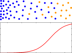 The dots along the top represent documents that were reviewed by a human, with relevant documents shown in orange and non-relevant documents shown in blue. As you move from left to right some feature that is a good indicator of relevance (meaning that it helps in distinguishing relevant documents from non-relevant documents) increases in frequency. For example, the frequency of a word like “fraud” might increase as you go to the right. The vertical position of the documents doesn’t matter — you can think of vertical position as specifying the frequency of a feature that is not a good indicator of relevance (e.g. the frequency of the word “office”). The algorithm is commonly given only yes/no values for relevance as input, so it has no way of knowing whether some of the orange documents are more important than others. What it does know is that a document has a higher probability of being relevant, assuming that the training set is representative of the document set in general, if it is farther to the right. The algorithm might even estimate the probability of a document being relevant based on how far to the right it is, as shown by the red curve below the dots.
When the algorithm is asked to make predictions for a document that has not been reviewed by a human, it can measure the frequency of the indicator word (e.g. “fraud”) for the document and spit out the probability estimate that was generated from the training data. Rather than the actual probability estimate, it could use any monotonic function of the probability estimate (i.e. any quantity that increases when the probability increases) as the relevance score.
Documents with a high relevance score are the documents that have the highest probability (as far as the algorithm can tell) of being relevant. They are the documents that the algorithm is confident are relevant. They are the low-hanging fruit if your goal is to find the largest number of relevant documents without wading through a lot of non-relevant documents. They are not necessarily the most informative or most relevant documents. Rather, they are the relevant documents that are easiest for the algorithm to find. Documents with a very low relevance score are the documents that have the lowest probability of being relevant. What about the documents between those extremes? Those are the documents where the algorithm just isn’t sure. The features that the algorithm uses to separate the documents that are relevant from those that aren’t simply don’t work well for those documents. Actual relevance for those documents may depend on words that the algorithm isn’t paying attention to, or it may depend on a very specific ordering of the words when the algorithm is ignoring word order, or it may depend on a subtle contextual detail that only a human could appreciate.
The relevance score indicates how well the algorithm understands the document based on experience with other similar documents in the training set, so it is clearly specific to the algorithm and is not an inherent property of the document. Different algorithms will do a better/worse job of finding features that separate relevant documents from non-relevant documents, and different algorithms will do a better/worse job of modeling the probability of a document being relevant based on experience with the training set. All of these things will impact the precision-recall curve.
At this point, the difference between an algorithm that produces a relevance score and an algorithm that produces a yes/no relevance prediction should be clear. An algorithm that produces a score “knows what it doesn’t know,” while an algorithm that produces a yes/no doesn’t (or it knows and refuses to tell you). An algorithm that produces a score tells you which documents it is uncertain about. You could always convert a score to a yes/no by picking an arbitrary cutoff for the score, say 50, and proclaiming that only documents reaching that threshold are predicted to be relevant. So, two documents with scores of 49 and 50, which might even be near-dupes, would be predicted to be non-relevant and relevant respectively. That should make the arbitrariness of a yes/no result clear. Whenever you produce a yes/no result, even if it doesn’t involve an explicit score and cutoff, there will be the possibility that two very similar documents will generate completely different outputs because a binary output does not allow the similarity of the inputs to be expressed.
If you are the producing party in a case, and you plan to review all documents before producing them, you can produce the largest number of responsive documents (one can certainly debate whether that is the most appropriate goal) at the lowest cost by ordering the documents by the relevance score to bring the low-hanging fruit to the top. As you work your way down the document list, you will have to review more and more non-responsive documents for each responsive document you hope to find (think about going from right to left in the diagram above). As described in my previous article, you can compute how many documents you’ll need to review to achieve a desired level of recall using the precision-recall curve, and the appropriate stopping point (recall level) for the case can be determined from proportionality and the cost curve. If the algorithm produces a yes/no prediction instead of a relevance score, you won’t have a precision-recall curve, just a single precision-recall point. The stopping point will be dictated by the software rather than proportionality and the value of the case.
Sidenote: The diagram shows the simplest possible example to illustrate the ideas in the article. It is, in fact, so simple that it would apply equally well to a keyword search for a single word if the search algorithm used word frequency to order the search results (many do). A more realistic example would involve many dimensions and relevance score contours that could not be achieved with a search engine, but the idea still holds — middling scores should occur for documents that reside in areas of the document space where relevant and non-relevant documents aren’t well-separated.
The Laguna Beach eDiscovery Retreat is part of The eDiscovery Retreats series put together by Chris La Cour. The venue was beautiful, with carefully maintained gardens and flowers, and a relaxing view of the ocean. You can see all of my photos of the resort and the surrounding area here.
There was a reception in the garden area on Sunday night. Monday started with a continental breakfast and a keynote address by Kimberly Newman of Walmart. There were five hour-long time slots for sessions during the remainder of the day. Each time slot had two simultaneous sessions to choose from. Sessions featured several experts who were guided by questions asked by a moderator and sometimes the audience. Lunch was held on the lawn with a view of the ocean.
My notes on the sessions I attended are below. Keep in mind that I could only attend half of them because there were simultaneous sessions, and my notes only cover a small fraction of the information presented.
Keynote Address: eDiscovery Maturity and The Road to ASCLD Accreditation – Walmart has 50 petabytes of data, 10,000 IT associates (employees), 10 million emails per day, litigation holds on 100,000 associates, 9,000 pending claims, and typically 200 pending class actions. Some data is on hold for a decade or more. Should have ASCLD accreditation by November. They hope it will reduce the risk of sanctions and establish good faith efforts. They block access to social networks from corporate computers. Processes are different overseas due to differing laws (e.g., ownership of email).
Implementing a Successful In-House eDiscovery Program or Strategy – Difficult if you don’t have support from top management. Having a crisis is the quick way to get buy-in. Pfizer has a specific contact for each outside counsel and meetings to discuss e-discovery initiatives. Chevron chooses e-discovery systems and requires outside counsel to use them. They have written expectations for outside counsel. Google is careful to not allow outside counsel to do things that have implications down the road. Use service providers because the cost of keeping stuff behind the firewall is huge. Regarding the service provider relationship, Chevron has a long vetting process, and gives them data and tests the result. Will the provider be around in three years? Have an SLA and a good contract. Establish a single point of contact. Make sure billing systems can match up. Pfizer is asking for fixed fee (not per-GB). Kia looks at references. Important to compare apples-to-apples on price — send pricing spreadsheet to vendors. Google wants vendors to tell them right away if there is any problem.
A Frank Conversation About the Meaning of Possession, Custody & Control – did not attend.
Organizing the Best eDiscovery “Team” – did not attend.
eDiscovery Goals – Don’t forget about the info your own client has. 72% of e-discovery is review. Less than 1% (or was it 0.1%?) of produced documents are marked for exhibit. Story of a firm that gave 1,200 requests for production (trying to harass into settlement). Another story of a firm that was sanctioned for overproducing to overwhelm the opponent. Don’t wait until the 26(f) to do due diligence. Cooperation may mean educating the other side. Judges don’t like discovery motions.
Ethics & Malpractice – did not attend.
EDD Project Management & Team Roles – More is being done in-house, so outside counsel has less knowledge about the case, which makes strategy hard. Outside counsel must certify the result, so communication is important. Company may contract with vendor directly to negotiate a price for e-discovery services (but outside counsel may have more knowledge about pricing in the market), so outside counsel may have to learn the chosen vendor’s process. Document review performed by a staffing agency can also result in outside counsel having less info about the case. Choose reviewers based on their expertise (privilege, pharmaceuticals, etc.). Look at reviewer speed — are they going too fast or too slow? Maybe they are not really trying, or are confused, or maybe they happen to be getting especially long/short documents.
Lit Holds & Collection – did not attend.
Search/Coding (Including Predictive Coding)/Analysis – I was on the panel, so I did not take notes.
Evolving Challenges in Electronic Discovery and Computer Forensics – If you don’t collect early, you may lose the opportunity to do it later (e.g., you can’t just copy a NAS). Collecting from Dropbox or iCloud – must be careful about ownership (personal vs. corporate). Dropbox stores encrypted cache on local computer. Dropbox keeps history log showing accesses – might find deletions. Use metadata to show that email or office document was forged. PDFs may retain info (botched redaction – just remove the black square hiding the text). Time stomping is changing the creation time for a file. Suspect time stomping when many of the documents have “000” for the milliseconds part of the time. Shellbags capture information about what is seen in Windows Explorer.
Use of Discovery Data – did not attend.
When you try to quantify how similar near-duplicates are, there are several subtleties that arise. This article looks at three reasonable, but different, ways of defining the near-dupe similarity between two documents. It also explains the popular MinHash algorithm, and shows that its results may surprise you in some circumstances.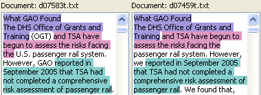 Near-duplicates are documents that are nearly, but not exactly, the same. They could be different revisions of a memo where a few typos were fixed or a few sentences were added. They could be an original email and a reply that quotes the original and adds a few sentences. They could be a Microsoft Word document and a printout of the same document that was scanned and OCRed with a few words not matching due to OCR errors. For e-discovery we want to group near-duplicates together, rather than discarding near-dupes as we might discard exact duplicates, since the small differences between near-dupes of responsive documents might reveal important information. Ideally, the document review software will display the near-dupes side-by-side with common text highlighted, as shown in the figure above, so reviewers don’t waste time reading the same text over and over. Typically, you’ll need to provide the near-dupe software with a threshold indicating how similar you want the documents to be in order for them to be grouped together. So, the software needs a concrete way to generate a number, say between 0 and 100%, measuring how similar two documents are. In this article we’ll look at some sensible ways of defining the near-dupe similarity.
The first two methods for measuring similarity involve identifying matching chunks of text in the documents. Suppose we have two documents with the shorter document having length S, measured by counting words (it would be more proper to say “tokens” instead of “words” since we might count numbers appearing in the text, too), and the longer document having length L. We identify substantial chunks of text (not just an isolated word or two) that the two documents have in common, and find the number of words in the common text that the documents share to be C. We could define the near-dupe similarity of the two documents to be (SL is the similarity, not to be confused with S, the length of the shorter document):
Since the number of words the documents have in common, C, cannot be larger than the number of words in either document, the ratio C/L is between 0 and 1 (the ratio C/S is also between 0 and 1, but you could have C/S=1 for documents of wildly different lengths if the short document is contained within the long one, so we don’t consider C/S to be a good measure for near-dupes, although it might be useful for other purposes). We can multiply by 100 to turn it into a percentage. Suppose we measure SL to be 80% for a pair of documents. That tells us that if we read either document we’ve read at least 80% of the content from the other document, so SL has a very practical meaning when it comes to making decisions about which documents you need to review. SL does have a shortcoming, however. It doesn’t depend on the length of the shorter document at all. If three documents have the same text in common, the value of SL will be the same when comparing the longest document to either of the two shorter ones, giving no hint that one of the shorter documents may contain more unique (not shared with the longest document) text than the other.
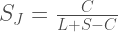
A different way of measuring the similarity is inspired by the Jaccard index from set theory:
The denominator may look a little strange, but it is just the amount of unique text contained in the combination of both documents. L+S is the total amount of text, but that counts the common chunks of text shared by both documents twice, so we subtract C to compensate for that double-counting. SJ is between 0 and 1. Note that SJ ≤ SL because the denominator for SJ is never smaller than the denominator for SL. To see that, note that the denominator for SJ has an extra S–C compared to the denominator for SL, and S–C is always greater than or equal to 0 because the amount of text the documents have in common is at most the length of the shorter document, i.e. S ≥ C. So, SJ is a somewhat pessimistic measure of how much the documents have in common. Let’s look at an example:

Example 1: Highlighted text is identical, so we don’t need to read it twice during review. L=100, S=97, C=85.
In Example 1 above, there are two chunks of text that match, one highlighted in orange and the other highlighted in blue. The matching chunks are separated by a single word where a typo was corrected (“too” and “to” don’t match). We have L=100, S=97, and C=85. Using the equations above we compute the two similarity measures to be SL=85% and SJ=76%.
Example 1 was pretty straightforward. Let’s consider a more challenging example:

Example 2: The document on the right is just two copies of the document on the left pasted together.
In Example 2, the document on the right contains two copies of the text from the document on the left pasted together. Forget the formulas and answer this question: What result would you want the software to give for the near-dupe similarity of these two documents? One approach, which I will call literal matching, requires a one-to-one matching of the actual text. It would view these documents as being 50% similar because only half of the document on the right matches up with text from the document on the left (SL and SJ are equal when all of the text from the short document matches with the long document, so there is no need to specify which similarity measure is being discussed in this case). A different approach, which I will call information matching, views these documents as a 100% match because duplicated chunks of text within the same document aren’t counted since they don’t add any new information. It’s as if the second copy of the sentence in the document on the right doesn’t exist because it adds nothing new to the document. You may be thinking that Example 2 is rather contrived, but repeated text within a document can happen if spreadsheets or computer-generated reports contain the same heading repeated on many different pages. So, what do you think is the most sensible approach for e-discovery purposes, literal matching or information matching? We’ll return to this issue later.
I said earlier that we are looking for “substantial” chunks of text that match between near-dupe documents, but I wasn’t explicit about what that means. I’m going to take it to mean at least five consecutive matching words for the remainder of this article. Five is an arbitrary choice that is not necessarily optimal, but it will suffice for the examples presented.
Example 3: Two potential matching chunks of text overlap in the document on the left. L=15, S=9, C=?
In Example 3, there are two 5-word-long chunks of text that could match between the two documents, but they overlap in the document on the left. The literal matching approach would say there are 5 words in common because matching “I will need money and” takes that chunk of words off the table for any further matching, leaving only 4 words (“cigars for the mayor”) remaining, which isn’t enough for a 5-word-long match. The information matching approach would say there are 9 words in common because all of the words in the document on the left are present in the document on the right in sufficiently large chunks.
So far, we’ve focused on similarity measures that require identification of matching chunks of text, but that can be algorithmically difficult. The third approach we’ll consider bases the similarity on counting shingles, i.e. overlapping contiguous sets of words of a specific length. The shingle-counting approach allows for use of a probabilistic trick called the MinHash algorithm to reduce memory consumption and speed up the calculation. I’ve seen virtually no discussion of the near-dupe algorithms used in e-discovery, but I suspect that shingling and MinHash are used by many tools because the approach is efficient and well-known (Clustify does not use this approach). MinHash is often discussed in the context of finding near-dupes of webpages. If you did a search on Google you would not want to see hundreds copies of the same Associated Press article that was syndicated to hundreds of websites (with slightly different header/footer text on each webpage) in the results, so search engines discard near-dupes. E-discovery can involve documents that are much shorter than webpages (e.g., emails), and the goal is to group near-dupes rather than discard them, so one should not assume that algorithms or minimum similarity thresholds designed for web search engines are appropriate for e-discovery.
To see what shingles look like, here are the 5-word shingles (there are 93 of them) for the document on the left in Example 1:
| 1 | It is important to use |
| 2 | is important to use available |
| 3 | important to use available technologies |
| 4 | to use available technologies to |
| … | |
| 92 | LLP and an expert on |
| 93 | and an expert on ediscovery |
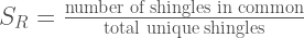
To compute the similarity, generate the shingles for the two documents being compared and count the number of shingles that are common to both documents and the total number of unique shingles across both documents and use the formula:
This is sometimes called the resemblance. Using 5-word shingles ensures that matching chunks of text must be at least five words long to contribute to the similarity. When counting shingles containing w words it is useful to note that a chunk of text containing N words will have N-(w-1) shingles. For the sake of comparison, it is useful to write SR in terms of the same word counts used in our other similarity measures. If the documents being compared have n chunks of text in common, we find the relationship:
The mess in square brackets in the rightmost part of the equation can be shown to be less than or equal to one (the proof is trivial for all cases except n=1, which is still pretty easy when you realize that C ≤ L+S–C). It is important to note that if we use the MinHash algorithm it will be impossible know n, so we cannot use the equation above to convert MinHash measurements of SR into SJ — we are stuck with SR as our similarity measure if we use MinHash. The relationship between our three similarity measures is:
Let’s compute SR for Example 1. We have n=2, w=5, L=100, S=97, and C=85, giving SR=69% (compared to SJ=76% and SL=85%). As you can see, it is important to know how the similarity is calculated when choosing a similarity threshold since values can vary significantly depending on the algorithm.
How bad can the disagreement between similarity measures be? The equation shows that SR differs from SJ most significantly when the average size of a matching hunk of text, C/n, is not much larger than the shingle size, w. Consider this example of an email and its reply:
Example 4: An email and its reply. Shows that short documents give very low similarity values when counting shingles. Also shows why it is important to group near-dupes rather than discarding them (don’t discard the confession!).
The email on the left is only five words long, so it has only one 5-word shingle. The reply on the right adds just one more word, so it has two shingles. We have a total of two unique shingles across both documents, and one shingle in common, so SR is 1/2=50% while SJ is 5/6=83%. Matching the first five words in the document on the right only counts as one common shingle, while failing to match just one word (the “Yes”) in the last five words in the document on the right counts as a non-matching shingle. This may seem like a defect, but it’s not as crazy as it might seem. Consider the contribution to the numerator of the similarity calculation for matching chunks of text of various lengths:
| Impact on Numerator of similarity | ||
|---|---|---|
| Number of Matching Words in chunk | SJ | SR |
| 3 | 0 | 0 |
| 4 | 0 | 0 |
| 5 | 5 | 1 |
| 6 | 6 | 2 |
| 7 | 7 | 3 |
| … | ||
| 100 | 100 | 96 |
For SJ, a match of four contiguous words counts for nothing, but a match of five words counts for five. Such an abrupt transition could be seen as undesirable. Shingle counting gives a much smoother transition for SR. You could view matching with 5-word shingles as saying: “We’ll count a 5-word match for something, but we really only take a match seriously if it is considerably longer than five words.”
So far, I’ve glossed over the issue of the same shingle appearing multiple times in the same document. We’ll see below that the MinHash algorithm effectively discards any duplicate shingles within a document. Recalling the terminology introduced earlier, SR with MinHash is an information matching approach, not a literal matching approach. Sort of, but not quite. Let’s return to Example 2, where the document on the right consisted of two sentences that were identical. The shingles covering the second sentence will be the same as those from the first sentence, so they won’t count, but the shingles that straddle the two sentences, starting toward the end of the first sentence and ending toward the beginning of the second sentence, are unique and will count. The document on the left contains 12 shingles that are all matched by the document on the right. The document on the right has an additional 4 shingles that straddle the boundary between the first and second sentence (e.g. “human reviewers. Predictive coding uses”), giving a total of 16 unique shingles. So SR is 12/16=75%. I challenged you earlier to decide what result you would want the software to give for Example 2, proposing 50% and 100% as two plausible values. How do you feel about 75%? If the repeated text was longer, SR would be closer to 100%.
Recall that Example 3 raised the issue of matching overlapping chunks of text. Shingle counting will happily match text that overlaps, but you should keep in mind that shingles that straddle two different matching chunks won’t match. There are 2 matching shingles in Example 3 (the text highlighted in orange and the text highlighted in blue). The document on the left has 5 shingles (including the two it has in common with document on the right) and the document on the right has 11 shingles, so SR is only 2/(5+11-2)=14%.
Finally, let’s look at the MinHash algorithm. Suppose the documents we are comparing are 3000 words long (roughly five printed pages). If we use 5-word shingles, that’s 2996 shingles per document that we need to store and compare, which would be pretty demanding if our document sent contained millions of documents. MinHash reduces the amount of data that must be stored and compared in exchange for giving a result that is only an approximation of SR. Suppose we listed all of the unique shingles from the two documents we wanted to compare and picked one of the shingles at random. What is the probability that the selected shingle would be one that is common to both documents? You would find that probability by dividing the number of common shingles by the total number of unique singles, but that’s exactly what we defined SR to be. So, we can estimate SR by estimating the probability that a randomly selected shingle is one that the documents share, which we can do by selecting shingles randomly and recording whether or not they are common to both documents; SR is then approximated by the number of common shingles we encountered divided by the number of shingles we sampled. If we sample a few hundred shingles, we’ll get an estimate for SR that is accurate to within plus or minus something like 7% (whether it is 7% or some other value depends on the number of selected samples and the desired confidence level — 200 samples at 95% confidence gives plus or minus 7%). It is tough to get the error bar on our similarity estimate much smaller than that because of the way error bars on statistically sampled values scale — to cut the error bar in half we would need four times as many samples. You can skip forward to the concluding paragraph at this point if you don’t want to read about the gory details of the MinHash algorithm; from a user’s point of view the critical thing to know is that the result is only an estimate.
MinHash uses a method of shingle sampling that is not truly random, but it is “random looking” in all ways that matter. The non-random aspect of the sampling is what allows it to reduce the amount of storage required. The MinHash algorithm computes a hash value for each shingle, and selects the shingle that has the smallest hash value. A hash function generates a number, the hash value, from a string of text in a systematic way such that the tiniest change in the text causes the hash value to be completely different. There is no obvious pattern to the hash values for a good hash function. For example, 50% of strings starting with the letter “a” will have a higher hash value than a string starting with the letter “b” — the hash value is not related to alphabetic ordering. So, selecting the shingle with minimum hash value is a “random looking” choice — it’s not at all obvious in advance which shingle will be chosen, but it is not truly random since the same hash function will always choose the same shingle. If we want to sample 200 shingles to estimate SR, we’ll need 200 different hash functions. Here is an example of hash values from two different hash functions applied to the shingles from the left document from Example 1:
| Shingle | hash1 | hash2 |
|---|---|---|
| It is important to use | 10419538473912939328824564064987594243 | 300214285342720760039511832324050800711 |
| is important to use available | 105555457340479730793594838617716806364 | 331180212539788074185988416231900930236 |
| important to use available technologies | 249315758303188756469411716170892733328 | 183376530549503672061864557636756469089 |
| to use available technologies to | 289630855896414368089666086343852687888 | 199563112601716758234064918560089655690 |
| … | ||
| LLP and an expert on | 54122989796249388067356565700270998745 | 298602506386019811335232493333781440033 |
| and an expert on ediscovery | 191435127605053759280177207148206634957 | 59413317844173777786126651204968182610 |
As you can see, the hash values have a lot of digits. For a good hash function, the probability of two different strings of text having the same hash value is extremely small (i.e. all of those digits really are meaningful, so the number of possible hash values is huge), so it’s pretty safe to assume that equal hash values implies identical text. That means we don’t need to store and compare the shingles themselves — we can store and compare the hash values instead.
The final, critical step in the MinHash algorithm is to reorganize our approach to finding the shingle (across both documents) with the minimum hash value and checking to see whether or not it is common to both documents. An equivalent approach is to find the minimum hash value for the shingles of each document separately. If those two minimum hash values (one for each document) are equal, it means the shingle having the minimum hash value across both documents exists in both documents (remember, equal hash values implies that the text is identical). If the two minimum hash values are different, it means the shingle having the minimum hash value across both documents exists in only one of the documents. This is where we get our huge performance boost. If we are comparing documents that are 3000 words long, we no longer need to store 2996 shingles (or hashes of the shingles) for each document and do a big comparison between two sets of 2996 shingles from the two documents we want to compare — we just need to compute the minimum hash value for each document once (not each time we do a comparison) and store that. When we want to compare the documents, we just compare that stored minimum hash value to see if it is equal for the two documents. So, our full procedure of “randomly” picking 200 shingles and measuring the percentage that appear in both documents to estimate SR (to within plus or minus 7%) boils down to finding the minimum hash value for each document for 200 different hash functions and storing those 200 minimum hash values, and estimating SR by counting the percentage of those 200 corresponding values that are equal for the two documents. Instead of storing the full document text, we merely need to store 200 hash values (computers store numbers more compactly than you might guess from all of the digits shown in the hash values above — those hash values only require 16 bytes of memory each).

Each document from Example 1 is represented by a circle. Shingles shown in the intersection are common to both documents. Only a subset of shingles are shown due to space constraints. Result of two hash functions being applied to shingles is shown with the last 34 digits of hash values dropped. Minimum hash value for each document is circled in orange. The first hash function selects a shingle common to both documents (“It is important to use”). The second hash function selects a shingle (“six years of experience in”) that exists only in the right document (minimum hash values for the individual documents don’t match).
As mentioned earlier, duplicated shingles within a document really only count once when using the MinHash algorithm. The duplicated shingles would just result in the same hash value appearing more than once, but that has no impact on the minimum hash value that is actually used for the calculation.
In conclusion, near-dupes aren’t as simple as one might expect, and it is important to understand what your near-dupe software is doing to ensure you are setting the similarity threshold appropriately and getting the results you expect. When doing document review with grouped near-dupes, you would like to tag all near-dupes of a non-responsive document as non-responsive without review while reviewing near-dupes of a responsive document in more detail. If misunderstandings about how the algorithm works cause the similarity values generated by the software to be higher than you expected when you chose the similarity threshold, you risk tagging near-dupes of non-responsive documents incorrectly (grouped documents are not as similar as you expected). If the similarity values are lower than you expected when you chose the threshold, you risk failing to group some highly similar documents together, which leads to less efficient review (extra groups to review). We examined three different, plausible measures of near-duplicate similarity. We found the relationship SR ≤ SJ ≤ SL, which is exemplified in our results from Example 1 where we calculated SR=69%, SJ=76% and SL=85% for a fairly normal pair of documents. Different similarity measures can disagree more significantly for short documents or documents where the same text is duplicated many times within the same document. We saw that the MinHash algorithm is an efficient way to estimate SR, but that estimate comes with an error bar. For example, an estimate of 69% means that the value is really (with 200 samples and 95% confidence) somewhere between 62% and 76%. Choosing an appropriate shingle size is important when computing SR. Large values for SR are only possible if the average chunk of matching text is significantly longer than the shingle size, which means that it is impossible to group very short (relative to the shingle size) documents (aside from exact dupes) using SR unless the minimum similarity threshold is set very low.
If you are planning to implement minhash, you can find a useful discussion on how to generate many hash functions here.
The press release announcing Clustify 3.2 went out yesterday. In this post I’ll talk a bit more about some of the features in the new version and provide some screenshots.

Keyword view for news articles from 2008. Lines connect words that are highly correlated. Groups of highly correlated words are given the same color to highlight main themes.
The biggest addition is the ability to export an SVG file that provides an interactive graphical visualization of the keyword and cluster relationships that can be viewed in a web browser. This is useful for getting a quick sense of the major themes in the document set and seeing which keywords are closely related to each other. You can configure it to link the clusters and keywords to an arbitrary URL with the ID of the clicked cluster or keyword embedded in the URL, so you can link a cluster or keyword to a browser-based review platform to display a list of documents from the clicked cluster or containing the clicked keyword.

Cluster view after clicking “Obama” from the keyword view. Hovering the mouse over “Hillary” highlights clusters labeled with that word.
Version 3.2 also adds the ability to export tags into virtually any database having an ODBC driver (Microsoft SQL Server, Oracle, DB2, MySQL, PostgreSQL, etc.) as additional columns. There is one column for each exported tag, containing “y” or “n” to indicate whether that tag was applied to the document. Tagging can be done more efficiently in Clustify than in many review platforms because you can tag entire clusters, or all clusters labeled with a particular combination of keywords, with a single mouse click or key-press. The addition of tag export allows you to export the tags from Clustify to virtually any review platform based on a standard database. This makes it practical to do full tagging within Clustify, or to do very crude tagging within Clustify to prioritize the documents for full review in a review platform.
The new version contains many smaller feature additions like the “Literal Jaccard” similarity function, the ability to sort clusters on any field in any context, and improvements to the algorithm for detecting email footers so they can be ignored (to avoid grouping emails together merely because they contain the same confidentiality notice). It also adds two new command-line tools, clustify_svg_creator (create graphical visualization) and clustify_match_highlighter (create side-by-side near-dupe comparison in HTML) , to allow users to tap into Clustify’s capabilities from within other programs without the Clustify GUI getting in the way.
According to the Infosecurity article ISO approves eDiscovery standards development, an international standard is being developed that “addresses terminology, provides an overview of eDiscovery and ESI, and then addresses a range of technological and process challenges.” The first working draft is due in early July, with comments on the draft due in early September. A linked article in Enterprise Communications elaborates that “The standard will also look to clarify any issues that aren’t directly dealt with in the Federal Rules of Civil Procedure.”
This is certainly an interesting development. Since it is an international standard, it will be challenging to make it compatible with many different bodies of law. Are they really doing something different from what EDRM already does? Will it get much buy-in from the courts and practitioners in the field?
Here are some brief highlights from today’s webinar on proposed changes to the Federal Rules of Civil Procedure held by the eDiscovery Education Center and sponsored by LexisNexis. The speakers were Michael R. Arkfeld, Judge John M. Facciola, Craig D. Ball, and Sean R. Gallagher. The webinar was an hour long and packed with information and opinions — this is just a small sample. The full webinar will be available for purchase within two weeks here.
The proposed changes will be open for public comment August through February. The earliest that the new rules could go into effect is December 2015. Gallagher encouraged people to get involved, and said the rules are still in play.
Proposed changes to 37(e) on failure to preserve discoverable information attempt to provide more clarity on the issue of sanctions. Facciola said that fear of sanctions caused people to preserve everything. The changes contemplate curative measures and provide factors for assessing the party’s conduct before imposing serious sanctions. Ball said nobody has been seriously sanctioned in the past for making a good faith effort that went awry, but the new rules will put and end to hand wringing over the possibility of severe sanctions over negligence without willful misconduct. Gallagher said the really egregious cases get the most attention, but the challenge is to create rules for more ordinary cases. Litigants will find more comfort in having national rules instead of applying results from cases from different jurisdictions.
Ball raised the point that the new rules don’t seem to provide for sanctions if a party tries to destroy evidence but is unsuccessful in doing so. Arkfeld questioned whether the rules would make sanctions more complicated to determine. Facciola didn’t think so since the factors are easy to apply, and he said making them explicit eases the pain for everyone. He said there have been some complaints because “anticipation of litigation” isn’t defined, but that would be too hard to do. Gallagher said there have been similar concerns about “willful.” Arkfeld asked whether the proposed change would give a pass to organizations so they don’t have to invest in controlling their ESI. Ball said there is some concern, but the new rule doesn’t fundamentally change what judges were already doing.
Proposed changes to rule 26(b)(1) involve addition of language about proportionality and removal of language about discovery of inadmissible information that might reasonably be expected to lead to discovery of admissible evidence. Facciola said this change is extremely important. Ball was somewhat less excited about it, and raised concerns about whether meta data and information about companies’ IT systems would no longer be discoverable. Gallagher was surprised that there hasn’t been more comment on the changes to rule 26, and thought there would be complaints in the future about the part that was removed.
Facciola said the language about proportionality was a technical change where things were moved around to make it clear that all discovery is subject to proportionality. Gallagher thought that change would be significant to litigants, with more litigation over the meaning of proportionality and how it is applied, but that’s not necessarily a bad thing since things will become more efficient over the long-term. Ball agreed and expressed concern about the possibility of litigants using their own interpretation of proportionality to limit the amount of preservation they do. He warned that proportionality should be based on the opinion of a judge who is well-informed about the case, not the producing party’s opinion.
This article describes how to measure the performance of predictive coding algorithms for categorizing documents. It describes the precision and recall metrics, and explains why the F1 score (also known as the F-measure or F-score) is virtually worthless.
Predictive coding algorithms start with a training set of example documents that have been tagged as either relevant or not relevant, and identify words or features that are useful for predicting whether or not other documents are relevant. “Relevant” will usually mean responsive to a discovery request in litigation, or having a particular issue code, or maybe privileged (although predictive coding may not be well-suited for identifying privileged documents). Most predictive coding algorithms will generate a relevance score or rank for each document, so you can order the documents with the ones most likely to be relevant (according to the algorithm) coming first and the ones most likely to not be relevant coming toward the end of the list. If you apply several different algorithms to the same set of documents and generate several ordered lists of documents, what quantities should you compute to assess which algorithm made the best predictions for this document set?
You could select some number of documents, n, from the top of each list and count how many of the documents truly are relevant. Divide the number of relevant documents by n and you have the precision, i.e. the fraction of selected documents that are relevant. High precision is good since it means that the algorithm has done a good job of moving the relevant documents to the top of the list. The other useful thing to know is the recall, which is the fraction of all relevant documents in the document set that were included in the algorithm’s top n documents. Have we found 80% of the relevant documents, or only 10%? If the answer is 10%, we probably need to increase n, i.e. select a larger set of top documents, if we are going to argue to a judge that we’re making an honest effort at finding relevant documents. As we increase n, the recall will increase each time we encounter another document that is truly relevant. The precision will typically decrease as we increase n because we are including more and more documents that the algorithm is increasingly pessimistic about. We can measure precision and recall for many different values of n to generate a graph of precision as a function of recall (n is not shown explicitly, but higher recall corresponds to higher n values — the relationship is monotonic but not linear). Click the graph to view the full-sized version:
 The graph shows hypothetical results for three different algorithms. Focus first on the blue curve representing the first algorithm. At 10% recall it shows a precision of 69%. So, if we work our way down from the top of the document list generated by algorithm 1 and review documents until we’ve found 10% of the documents that are truly relevant, we’ll find that 69% of the documents we encounter are truly relevant while 31% are not relevant. If we continue to work our way down the document list, reviewing documents that the algorithm thinks are less and less likely to be relevant, and eventually get to the point where we’ve encountered 70% of the truly relevant documents (70% recall), 42% of the documents we review along the way will be truly relevant (42% precision) and 58% will not be relevant.
Turn now to the second algorithm, which is shown in green. For all values of recall it has a lower precision than the first algorithm. For this document set it is simply inferior (glossing over subtleties like result diversity) to the first algorithm — it returns more irrelevant documents for each truly relevant document it finds, so a human reviewer will need to wade through more junk to attain a desired level of recall. Of course, algorithm 2 might triumph on a different document set where the features that distinguish a relevant document are different.
The third algorithm, shown in orange, is more of a mixed bag. For low recall (left side of graph) it has higher precision than any of the other algorithms. For high recall (right side of graph) it has the worst precision of the three algorithms. If we were designing a web search engine to compete with Google, algorithm 3 might be pretty attractive because the precision at low recall is far more important than the precision at high recall since most people will only look at the first page or two of search results, not the 1000th page. E-Discovery is very different from web search in that regard — you need to find most of the relevant documents, not just the 10 or 20 best ones. Precision at high recall is critical for e-discovery, and that is where algorithm 3 falls flat on its face. Still, there is some value in having high precision at low recall since it may help you decide early in the review that the evidence against your side is bad enough to warrant settling immediately instead of continuing the review.
You may have noticed that all three algorithms have 15% precision at 100% recall. Don’t take that to mean that they are in any sense equally good at high recall — they are actually all completely worthless at 100% recall. In this example, the prevalence of relevant documents is 15%, meaning that 15% of the documents in the entire document set are relevant. If your algorithm for finding relevant documents was to simply choose documents randomly, you would achieve 15% precision for all recall values. What makes algorithm 3 a disaster at high recall is the fact that it drops close to 15% precision long before reaching 100% recall, losing all ability to differentiate between documents that are relevant and those that are not relevant.
As alluded to earlier, high precision is desirable to reduce the amount of manual document review. Let’s make that idea more precise. Suppose you are the producing party in a case. You need to produce a large percentage of the responsive documents to satisfy your duty to the court. You use predictive coding to order the documents based on the algorithm’s prediction of which documents are most likely to be responsive. You plan to manually review any documents that will be produced to the other side (e.g., to verify responsiveness, check for privilege, perform redactions, or just be aware of the evidence you’ll need to counter in court), so how many documents will you need to review, including non-responsive documents that the algorithm thought were responsive, to reach a reasonable recall? Here is the formula (excluding training and validation sets):
The recall is the desired level you want to reach, and the precision is measured at that recall level. The prevalence is a property of the document set, so the only quantity in the equation that depends on the predictive coding algorithm is the precision at the desired recall. Here is a graph based on the precision vs. recall relationships from earlier:

If your goal is to find at least 70% of the responsive documents (70% recall), you’ll need to review at least 25% of the documents ranked most highly by algorithm 1. Keep in mind that only 15% of the whole document set is responsive in our example (i.e. 15% prevalence), so aiming to find 70% of the responsive documents by reviewing 25% of the document set means reviewing 10.5% of the document set that is responsive (70% of 15%) and 14.5% of the document set that is not responsive, which is consistent with our precision-recall graph showing 42% precision at 70% recall (10.5/25 = 0.42) for algorithm 1. If you had the misfortune of using algorithm 3, you would need to review 50% of the entire document set just to find 70% of the responsive documents. To achieve 70% recall you would need to review twice as many documents with algorithm 3 compared to algorithm 1 because the precision of algorithm 3 at 70% recall is half the precision of algorithm 1.
Notice how the graph slopes upward more and more rapidly as you aim for higher recall because it becomes harder and harder to find a relevant document as more and more of the low hanging fruit gets picked. So, what recall should you aim for in an actual case? This is where you need to discuss the issue of proportionality with the court. Each additional responsive document is, on average, more expensive than the last one, so a balance must be struck between cost and the desire to find “everything.” The appropriate balance will depend on the matter being litigated.
We’ve seen that recall is important to demonstrate to the court that you’ve found a substantial percentage of the responsive documents, and we’ve seen that precision determines the number of documents that must be reviewed (hence, the cost) to achieve a desired recall. People often quote another metric, the F1 score (also known as the F-measure or F-score), which is the harmonic mean of the recall and the precision:
The F1 score lies between the value of the recall and the value of the precision, and tends to lie closer to the smaller of the two, so high values for the F1 score are only possible if both the precision and recall are large.
Before explaining why the F1 score is pointless for measuring predictive coding performance, let’s consider a case where it makes a little bit of sense. Suppose we send the same set of patients to two different doctors who will each screen them for breast cancer using the palpation method (feeling for lumps). The first doctor concludes that 50 of them need further testing, but the additional testing shows that only 3 of them actually have cancer, giving a precision of 6.0% (these numbers are entirely made up and are not necessarily realistic). The second doctor concludes that 70 of the patients need further testing, but additional testing shows that only 4 of them have cancer, giving a precision of 5.7%. Which doctor is better at identifying patients in need of additional testing? The first doctor has higher precision, but that precision is achieved at a lower level of recall (only found 3 cancers instead of 4). We know that precision tends to decline with increasing recall, so the fact that the second doctor has lower precision does not immediately lead to the conclusion that he/she is less capable. Since the F1 score combines precision and recall such that increases in one offset (to some degree) decreases in the other, we could compute F1 scores for the two doctors. To compute F1 we need to compute the recall, which means that we need to know how many of the patients actually have cancer. If 5 have cancer, the F1 scores for the doctors will be 0.1091 and 0.1067 respectively, so the first doctor scores higher. If 15 have cancer, the F1 scores will be 0.0923 and 0.0941 respectively, so the second doctor scores higher. Increasing the number of cancers from 5 to 15 decreases the recall values, bringing them closer to the precision values, which causes the recall to have more impact (relative to the precision) on the F1 score.
The harmonic mean is commonly used to combine rates. For example, you should be able to convince yourself that the appropriate way to compute the average MPG fuel efficiency rating for a fleet of cars is to take the harmonic mean (not the arithmetic mean) of the MPG values of the individual cars. But, the F1 score is the harmonic mean of two rates having different meanings, not the same rate measured for two different objects. It’s like adding the length of your foot to the length of your arm. They are both lengths, but does the result from adding them really make any sense? A 10% change in the length of your arm would have much more impact than a 10% change in the length of your foot, so maybe you should add two times the length of your foot to your arm. Or, maybe add three times the length of your foot to your arm. The relative weighting of your foot and arm lengths is rather arbitrary since the sum you are calculating doesn’t have any specific use that could nail down the appropriate weighting. The weighting of precision vs. recall in the F1 score is similarly arbitrary. If you want to weight the recall more heavily, there is a metric called F2 that does that. If you want to weight the precision more heavily, F0.5 does that. In fact, there is a whole spectrum of F measures offering any weighting you want — you can find the formula in Wikipedia. In our example of doctors screening for cancer, what is the right weighting to appropriately balance the potential loss of life by missing a cancer (low recall) against the cost and suffering of doing additional testing on many more patients that don’t have cancer (higher recall obtained at the expense of lower precision)? I don’t know the answer, but it is almost certainly not F1. Likewise, what is the appropriate weighting for predictive coding? Probably not F1.
Why did we turn to the F1 score when comparing doctors doing cancer screenings? We did it because we had two different recall values for the doctors, so we couldn’t compare precision values directly. We used the F1 score to adjust for the tradeoff between precision and recall, but we did so with a weighting that was arbitrary (sometimes pronounced “wrong”). Why were we stuck with two different recall values for the two doctors? Unlike a predictive coding algorithm, we can’t ask a doctor to rank a group of patients based on how likely he/she thinks it is that each of them has cancer. The doctor either feels a lump, or he/she doesn’t. We might expand the doctor’s options to include “maybe” in addition to “yes” and “no,” but we can’t expect the doctor to say that one patient is a 85.39 score for cancer while another is a 79.82 so we can get a definite ordering. We don’t have that problem (normally) when we want to compare predictive coding algorithms — we can choose whatever recall level we are interested in and measure the precision of all algorithms at that recall, so we can compare apples to apples instead of apples to oranges.
Furthermore, a doctor’s ability to choose an appropriate threshold for sending people for additional testing is part of the measure of his/her ability, so we should allow him/her to decide how many people to send for additional testing, not just which people, and measure whether his/her choice strikes the right balance to achieve the best outcomes, which necessitates comparing different levels of recall for different doctors. In predictive coding it is not the algorithm’s job to decide when we should stop looking for additional relevant documents — that is dictated by proportionality. If the litigation is over a relatively small amount of money, a modest target recall may be accepted to keep review costs reasonable relative to the amount of money at stake. If a great deal of money is at stake, pushing for a high recall that will require reviewing a lot of irrelevant documents may be warranted. The point is that the appropriate tradeoff between low recall with high precision and high recall with lower precision depends on the economics of the case, so it cannot be captured by a statistic with fixed (arbitrary) weight like the F1 score.
Here is a graph of the F1 score for the three algorithms we’ve been looking at:

Remember that the F1 score can only be large if both the recall and precision are large. At the left edge of the chart the recall is low, so the F1 score is small. At the right edge the recall is high but the precision is typically low, so the F1 score is small. Note that algorithm 1 has its maximum F1 score of 0.264 at 62% recall, while algorithm 3 has its maximum F1 score of 0.242 at 44% recall. Comparing maximum F1 scores to identify the best algorithm is really an apples to oranges comparison (comparing values at different recall levels), and in this case it would lead you to conclude that algorithm 3 is the second best algorithm when we know that it is by far the worst algorithm at high recall. Of course, you might retort that algorithms should be compared by comparing F1 scores at the same recall level instead of comparing maximum F1 scores, but the F1 score would really serve no purpose in that case — we could just compare precision values.
In summary, recall and precision are metrics that relate very directly to important aspects of document review — the need to identify a substantial portion of the relevant documents (recall), and the need to keep costs down by avoiding review of irrelevant documents (precision). A predictive coding algorithm orders the document list to put the documents that are expected to have the best chance of being relevant at the top. As the reviewer works his/her way down the document list recall will increase (more relevant documents found), but precision will typically decrease (increasing percentage of documents are not relevant). The F1 score attempts to combine the precision and recall in a way that allows comparisons at different levels of recall by balancing increasing recall against decreasing precision, but it does so with a weighting between the two quantities that is arbitrary rather than reflecting the economics of the case. It is better to compare algorithm performance by comparing precision at the same level of recall, with the recall chosen to be reasonable for a case.
Note: You can read more about performance measures here, and there is an article on an alternative to F1 that is more appropriate for e-discovery here.

![S_R = \frac{C - n\times(w-1)}{L+S-C+(n-2)\times(w-1)} = S_J \times \left[\frac{1-\frac{n\times(w-1)}{C}}{1 + \frac{(n-2)\times(w-1)}{L+S-C}}\right]](https://s0.wp.com/latex.php?latex=S_R+%3D+%5Cfrac%7BC+-+n%5Ctimes%28w-1%29%7D%7BL%2BS-C%2B%28n-2%29%5Ctimes%28w-1%29%7D+%3D+S_J+%5Ctimes+%5Cleft%5B%5Cfrac%7B1-%5Cfrac%7Bn%5Ctimes%28w-1%29%7D%7BC%7D%7D%7B1+%2B+%5Cfrac%7B%28n-2%29%5Ctimes%28w-1%29%7D%7BL%2BS-C%7D%7D%5Cright%5D&bg=ffffff&fg=444444&s=2&c=20201002)


