This article describes how to measure the performance of predictive coding algorithms for categorizing documents. It describes the precision and recall metrics, and explains why the F1 score (also known as the F-measure or F-score) is virtually worthless.
Predictive coding algorithms start with a training set of example documents that have been tagged as either relevant or not relevant, and identify words or features that are useful for predicting whether or not other documents are relevant. “Relevant” will usually mean responsive to a discovery request in litigation, or having a particular issue code, or maybe privileged (although predictive coding may not be well-suited for identifying privileged documents). Most predictive coding algorithms will generate a relevance score or rank for each document, so you can order the documents with the ones most likely to be relevant (according to the algorithm) coming first and the ones most likely to not be relevant coming toward the end of the list. If you apply several different algorithms to the same set of documents and generate several ordered lists of documents, what quantities should you compute to assess which algorithm made the best predictions for this document set?
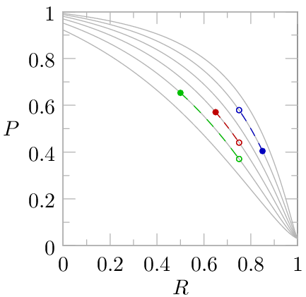
You could select some number of documents, n, from the top of each list and count how many of the documents truly are relevant. Divide the number of relevant documents by n and you have the precision, i.e. the fraction of selected documents that are relevant. High precision is good since it means that the algorithm has done a good job of moving the relevant documents to the top of the list. The other useful thing to know is the recall, which is the fraction of all relevant documents in the document set that were included in the algorithm’s top n documents. Have we found 80% of the relevant documents, or only 10%? If the answer is 10%, we probably need to increase n, i.e. select a larger set of top documents, if we are going to argue to a judge that we’re making an honest effort at finding relevant documents. As we increase n, the recall will increase each time we encounter another document that is truly relevant. The precision will typically decrease as we increase n because we are including more and more documents that the algorithm is increasingly pessimistic about. We can measure precision and recall for many different values of n to generate a graph of precision as a function of recall (n is not shown explicitly, but higher recall corresponds to higher n values — the relationship is monotonic but not linear). Click the graph to view the full-sized version:
 The graph shows hypothetical results for three different algorithms. Focus first on the blue curve representing the first algorithm. At 10% recall it shows a precision of 69%. So, if we work our way down from the top of the document list generated by algorithm 1 and review documents until we’ve found 10% of the documents that are truly relevant, we’ll find that 69% of the documents we encounter are truly relevant while 31% are not relevant. If we continue to work our way down the document list, reviewing documents that the algorithm thinks are less and less likely to be relevant, and eventually get to the point where we’ve encountered 70% of the truly relevant documents (70% recall), 42% of the documents we review along the way will be truly relevant (42% precision) and 58% will not be relevant.
Turn now to the second algorithm, which is shown in green. For all values of recall it has a lower precision than the first algorithm. For this document set it is simply inferior (glossing over subtleties like result diversity) to the first algorithm — it returns more irrelevant documents for each truly relevant document it finds, so a human reviewer will need to wade through more junk to attain a desired level of recall. Of course, algorithm 2 might triumph on a different document set where the features that distinguish a relevant document are different.
The third algorithm, shown in orange, is more of a mixed bag. For low recall (left side of graph) it has higher precision than any of the other algorithms. For high recall (right side of graph) it has the worst precision of the three algorithms. If we were designing a web search engine to compete with Google, algorithm 3 might be pretty attractive because the precision at low recall is far more important than the precision at high recall since most people will only look at the first page or two of search results, not the 1000th page. E-Discovery is very different from web search in that regard — you need to find most of the relevant documents, not just the 10 or 20 best ones. Precision at high recall is critical for e-discovery, and that is where algorithm 3 falls flat on its face. Still, there is some value in having high precision at low recall since it may help you decide early in the review that the evidence against your side is bad enough to warrant settling immediately instead of continuing the review.
You may have noticed that all three algorithms have 15% precision at 100% recall. Don’t take that to mean that they are in any sense equally good at high recall — they are actually all completely worthless at 100% recall. In this example, the prevalence of relevant documents is 15%, meaning that 15% of the documents in the entire document set are relevant. If your algorithm for finding relevant documents was to simply choose documents randomly, you would achieve 15% precision for all recall values. What makes algorithm 3 a disaster at high recall is the fact that it drops close to 15% precision long before reaching 100% recall, losing all ability to differentiate between documents that are relevant and those that are not relevant.
As alluded to earlier, high precision is desirable to reduce the amount of manual document review. Let’s make that idea more precise. Suppose you are the producing party in a case. You need to produce a large percentage of the responsive documents to satisfy your duty to the court. You use predictive coding to order the documents based on the algorithm’s prediction of which documents are most likely to be responsive. You plan to manually review any documents that will be produced to the other side (e.g., to verify responsiveness, check for privilege, perform redactions, or just be aware of the evidence you’ll need to counter in court), so how many documents will you need to review, including non-responsive documents that the algorithm thought were responsive, to reach a reasonable recall? Here is the formula (excluding training and validation sets):

The recall is the desired level you want to reach, and the precision is measured at that recall level. The prevalence is a property of the document set, so the only quantity in the equation that depends on the predictive coding algorithm is the precision at the desired recall. Here is a graph based on the precision vs. recall relationships from earlier:

If your goal is to find at least 70% of the responsive documents (70% recall), you’ll need to review at least 25% of the documents ranked most highly by algorithm 1. Keep in mind that only 15% of the whole document set is responsive in our example (i.e. 15% prevalence), so aiming to find 70% of the responsive documents by reviewing 25% of the document set means reviewing 10.5% of the document set that is responsive (70% of 15%) and 14.5% of the document set that is not responsive, which is consistent with our precision-recall graph showing 42% precision at 70% recall (10.5/25 = 0.42) for algorithm 1. If you had the misfortune of using algorithm 3, you would need to review 50% of the entire document set just to find 70% of the responsive documents. To achieve 70% recall you would need to review twice as many documents with algorithm 3 compared to algorithm 1 because the precision of algorithm 3 at 70% recall is half the precision of algorithm 1.
Notice how the graph slopes upward more and more rapidly as you aim for higher recall because it becomes harder and harder to find a relevant document as more and more of the low hanging fruit gets picked. So, what recall should you aim for in an actual case? This is where you need to discuss the issue of proportionality with the court. Each additional responsive document is, on average, more expensive than the last one, so a balance must be struck between cost and the desire to find “everything.” The appropriate balance will depend on the matter being litigated.
We’ve seen that recall is important to demonstrate to the court that you’ve found a substantial percentage of the responsive documents, and we’ve seen that precision determines the number of documents that must be reviewed (hence, the cost) to achieve a desired recall. People often quote another metric, the F1 score (also known as the F-measure or F-score), which is the harmonic mean of the recall and the precision:

The F1 score lies between the value of the recall and the value of the precision, and tends to lie closer to the smaller of the two, so high values for the F1 score are only possible if both the precision and recall are large.
Before explaining why the F1 score is pointless for measuring predictive coding performance, let’s consider a case where it makes a little bit of sense. Suppose we send the same set of patients to two different doctors who will each screen them for breast cancer using the palpation method (feeling for lumps). The first doctor concludes that 50 of them need further testing, but the additional testing shows that only 3 of them actually have cancer, giving a precision of 6.0% (these numbers are entirely made up and are not necessarily realistic). The second doctor concludes that 70 of the patients need further testing, but additional testing shows that only 4 of them have cancer, giving a precision of 5.7%. Which doctor is better at identifying patients in need of additional testing? The first doctor has higher precision, but that precision is achieved at a lower level of recall (only found 3 cancers instead of 4). We know that precision tends to decline with increasing recall, so the fact that the second doctor has lower precision does not immediately lead to the conclusion that he/she is less capable. Since the F1 score combines precision and recall such that increases in one offset (to some degree) decreases in the other, we could compute F1 scores for the two doctors. To compute F1 we need to compute the recall, which means that we need to know how many of the patients actually have cancer. If 5 have cancer, the F1 scores for the doctors will be 0.1091 and 0.1067 respectively, so the first doctor scores higher. If 15 have cancer, the F1 scores will be 0.0923 and 0.0941 respectively, so the second doctor scores higher. Increasing the number of cancers from 5 to 15 decreases the recall values, bringing them closer to the precision values, which causes the recall to have more impact (relative to the precision) on the F1 score.
The harmonic mean is commonly used to combine rates. For example, you should be able to convince yourself that the appropriate way to compute the average MPG fuel efficiency rating for a fleet of cars is to take the harmonic mean (not the arithmetic mean) of the MPG values of the individual cars. But, the F1 score is the harmonic mean of two rates having different meanings, not the same rate measured for two different objects. It’s like adding the length of your foot to the length of your arm. They are both lengths, but does the result from adding them really make any sense? A 10% change in the length of your arm would have much more impact than a 10% change in the length of your foot, so maybe you should add two times the length of your foot to your arm. Or, maybe add three times the length of your foot to your arm. The relative weighting of your foot and arm lengths is rather arbitrary since the sum you are calculating doesn’t have any specific use that could nail down the appropriate weighting. The weighting of precision vs. recall in the F1 score is similarly arbitrary. If you want to weight the recall more heavily, there is a metric called F2 that does that. If you want to weight the precision more heavily, F0.5 does that. In fact, there is a whole spectrum of F measures offering any weighting you want — you can find the formula in Wikipedia. In our example of doctors screening for cancer, what is the right weighting to appropriately balance the potential loss of life by missing a cancer (low recall) against the cost and suffering of doing additional testing on many more patients that don’t have cancer (higher recall obtained at the expense of lower precision)? I don’t know the answer, but it is almost certainly not F1. Likewise, what is the appropriate weighting for predictive coding? Probably not F1.
Why did we turn to the F1 score when comparing doctors doing cancer screenings? We did it because we had two different recall values for the doctors, so we couldn’t compare precision values directly. We used the F1 score to adjust for the tradeoff between precision and recall, but we did so with a weighting that was arbitrary (sometimes pronounced “wrong”). Why were we stuck with two different recall values for the two doctors? Unlike a predictive coding algorithm, we can’t ask a doctor to rank a group of patients based on how likely he/she thinks it is that each of them has cancer. The doctor either feels a lump, or he/she doesn’t. We might expand the doctor’s options to include “maybe” in addition to “yes” and “no,” but we can’t expect the doctor to say that one patient is a 85.39 score for cancer while another is a 79.82 so we can get a definite ordering. We don’t have that problem (normally) when we want to compare predictive coding algorithms — we can choose whatever recall level we are interested in and measure the precision of all algorithms at that recall, so we can compare apples to apples instead of apples to oranges.
Furthermore, a doctor’s ability to choose an appropriate threshold for sending people for additional testing is part of the measure of his/her ability, so we should allow him/her to decide how many people to send for additional testing, not just which people, and measure whether his/her choice strikes the right balance to achieve the best outcomes, which necessitates comparing different levels of recall for different doctors. In predictive coding it is not the algorithm’s job to decide when we should stop looking for additional relevant documents — that is dictated by proportionality. If the litigation is over a relatively small amount of money, a modest target recall may be accepted to keep review costs reasonable relative to the amount of money at stake. If a great deal of money is at stake, pushing for a high recall that will require reviewing a lot of irrelevant documents may be warranted. The point is that the appropriate tradeoff between low recall with high precision and high recall with lower precision depends on the economics of the case, so it cannot be captured by a statistic with fixed (arbitrary) weight like the F1 score.
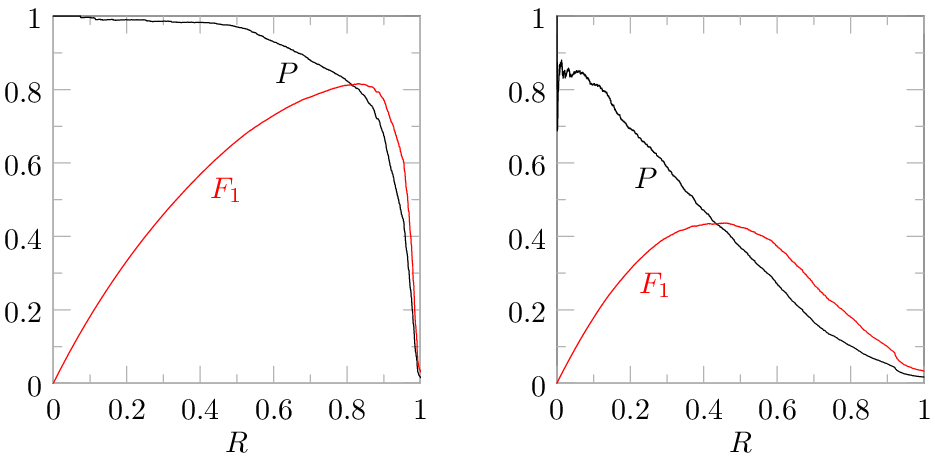
Here is a graph of the F1 score for the three algorithms we’ve been looking at:

Remember that the F1 score can only be large if both the recall and precision are large. At the left edge of the chart the recall is low, so the F1 score is small. At the right edge the recall is high but the precision is typically low, so the F1 score is small. Note that algorithm 1 has its maximum F1 score of 0.264 at 62% recall, while algorithm 3 has its maximum F1 score of 0.242 at 44% recall. Comparing maximum F1 scores to identify the best algorithm is really an apples to oranges comparison (comparing values at different recall levels), and in this case it would lead you to conclude that algorithm 3 is the second best algorithm when we know that it is by far the worst algorithm at high recall. Of course, you might retort that algorithms should be compared by comparing F1 scores at the same recall level instead of comparing maximum F1 scores, but the F1 score would really serve no purpose in that case — we could just compare precision values.
In summary, recall and precision are metrics that relate very directly to important aspects of document review — the need to identify a substantial portion of the relevant documents (recall), and the need to keep costs down by avoiding review of irrelevant documents (precision). A predictive coding algorithm orders the document list to put the documents that are expected to have the best chance of being relevant at the top. As the reviewer works his/her way down the document list recall will increase (more relevant documents found), but precision will typically decrease (increasing percentage of documents are not relevant). The F1 score attempts to combine the precision and recall in a way that allows comparisons at different levels of recall by balancing increasing recall against decreasing precision, but it does so with a weighting between the two quantities that is arbitrary rather than reflecting the economics of the case. It is better to compare algorithm performance by comparing precision at the same level of recall, with the recall chosen to be reasonable for a case.
Note: You can read more about performance measures here, and there is an article on an alternative to F1 that is more appropriate for e-discovery here.

 compares two different classification algorithms applied to the same task. To do a sensible comparison, we should compare precision values at the same level of recall. In other words, we should compare the cost of reaching equally good (same recall) productions. Furthermore, the recall level where the algorithms are compared should be one that is sensible for for ediscovery — achieving high precision at a recall level a court wouldn’t accept isn’t very useful. If we compare the two algorithms at R=75%, 1-NN has P=6.6% and 40-NN has P=70.4%. In other words, if you sort by relevance score with the two algorithms and review documents from top down until 75% of the relevant documents are found, you would review 15.2 documents per relevant document found with 1-NN and 1.4 documents per relevant document found with 40-NN. The 1-NN algorithm would require over ten times as much document review as 40-NN. 1-NN has been used in some popular TAR systems. I explained why it performs so badly in a previous article.
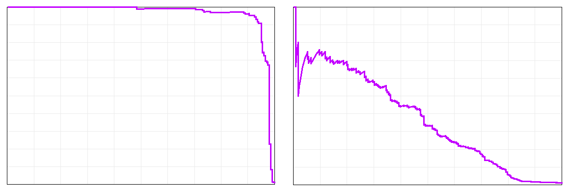
 which is the percentage of predictions that are correct. If a system predicts that none of the documents are relevant and prevalence is 10% (meaning 10% of the documents are relevant), it will have 90% accuracy because its predictions were correct for all of the non-relevant documents. If prevalence is 1%, a system that predicts none of the documents are relevant achieves 99% accuracy. Such incredibly high numbers for algorithms that fail to find anything! When prevalence is low, as it often is in ediscovery, accuracy makes everything look like it performs well, including algorithms like 1-NN that can be a disaster at high recall. The graph to the right shows the accuracy-recall curve that corresponds to the earlier precision-recall curve (prevalence is 2.633% in this case), showing that it is easy to achieve high accuracy with a poor algorithm by evaluating it at a low recall level that would not be acceptable for ediscovery. The maximum accuracy achieved by 1-NN in this case was 98.2% and the max for 40-NN was 98.6%. In case you are curious, the relationship between accuracy, precision, and recall is:

 I’ve criticized its use in ediscovery before. The relationship to precision and recall is: